Solutions for code challenges

Chapter 2

library(ggplot2)
v <- c(1, 2)
s <- rnorm(10)

all_vectors <- data.frame(xend = c(v[1], v[1] * s),
                          yend = c(v[2], v[2] * s),
                          Vector = c("Original", rep("Scaled", length(s))),
                          x = 0,
                          y = 0)

ggplot(data=all_vectors, aes(x=x, y=y, xend=xend, yend=yend, color=Vector)) + 
  geom_segment(arrow= arrow(length = unit(0.03, "npc"))) +
  xlim(-4, 4) +
  ylim(-4, 4) + 
  coord_equal()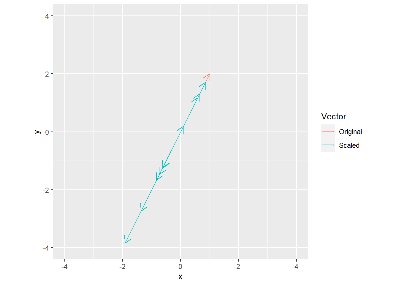

Chapter 3

Exercise 1

v1 <- c(1, 2, 3, 4, 5)
v2 <- c(2, 3, 4, 5, 6)
v3 <- c(3, 4, 5, 6, 7)
w <- c(-1, 3, 2)
result <- v1 * w[1] + v2 * w[2] + v3* w[3]

Exercise 2

v <- c(7, 4, -5, 8, 3)
o <- rep(1, length(v))
ave <- pracma::dot(v, o) / length(v)

Exercise 3

v <- c(7, 4, -5, 8, 3)
w <- runif(length(v))
wAve <- pracma::dot(v, w / sum(w))

Chapter 5

Exercise 1

A <- matrix(runif(n=4*2), nrow=4, ncol=2)
B <- matrix(runif(n=4*2), nrow=4, ncol=2)
C <- matrix(NA, nrow=2, ncol=2)
for(coli in 1:2){
  for(colj in 1:2){
    C[coli, colj] <- pracma::dot(A[, coli], B[, colj])
  }
}

Exercise 2

A <- matrix(runif(n=4*4), nrow=4, ncol=4)
Al <- pracma::tril(A)
S <- Al + t(Al)

Exercise 3

D <- matrix(0, nrow=4, ncol=8)
for(d in 1:min(dim(D))){
  D[d, d] <- d
}

# or
D <- diag(1:4, nrow=4, ncol=8)

Chapter 6

Exercise 1

A <- matrix(runif(n=2*4), nrow=2, ncol=4)
B <- matrix(runif(n=4*3), nrow=4, ncol=3)
C1 <- matrix(0, nrow=2, ncol=3)
for(i in 1:4){
  C1 <- C1 + outer(A[, i], B[i, ])
}
C1 - A %*% B

##      [,1] [,2] [,3]
## [1,]    0    0    0
## [2,]    0    0    0

Exercise 2

D <- diag(1:4)
A <- matrix(runif(n=4*4), nrow=4, ncol=4)
C1 <- D * A
C2 <- D %*% A
print(diag(C1))

## [1] 0.9799352 1.2875747 0.1189195 3.8517034

print(diag(C2))

## [1] 0.9799352 1.2875747 0.1189195 3.8517034

Exercise 3

A <- diag(runif(3))
C1 <- (t(A) + A) / 2
C2 <- t(A) %*% A
C1 - sqrt(C2)

##      [,1] [,2] [,3]
## [1,]    0    0    0
## [2,]    0    0    0
## [3,]    0    0    0

Exercise 4

Note that norm() requires a matrix as an input, therefore, we convert an atomic vector to a matrix for the norm computation.

m <- 5
A <- matrix(runif(n=m*m), nrow=m, ncol=m)
v <- runif(n=m)
LHS <- norm(A %*% v, type = "F")
RHS <- norm(A, type = "F") * norm(matrix(v), type="F")
RHS - LHS # should always be positive

## [1] 0.7464557

Chapter 7

Exercise 1

A <- matrix(runif(n=9*2), nrow=9, ncol=2)
B <- matrix(runif(n=2*16), nrow=2, ncol=16)
C <- A %*% B

Exercise 2

Z <- matrix(0, nrow=5, ncol=5)
N <- matrix(runif(5 * 5), nrow=5, ncol=5)
ZN <-  Z + N * .Machine$double.eps * 1e-307
print(pracma::Rank(Z))

## [1] 0

print(pracma::Rank(ZN))

## Warning in pracma::Rank(ZN): Rank calculation may be problematic.

## [1] 5

print(norm(ZN, type = "F"))

## [1] 6.422853e-323

Chapter 8

Exercise 1

A <- matrix(runif(n=4*3), nrow=4, ncol=3) %*% matrix(runif(n=3*4), nrow=3, ncol=4)
B <- matrix(runif(n=4*3), nrow=4, ncol=3) %*% matrix(runif(n=3*4), nrow=3, ncol=4)
n <- pracma::nullspace(A)
print(B %*% A %*% n) # zeros vector

##              [,1]
## [1,] 2.220446e-16
## [2,] 4.440892e-16
## [3,] 3.330669e-16
## [4,] 2.220446e-16

print(A %*% B %*% n) # not zeros vector

##           [,1]
## [1,] 0.4645256
## [2,] 1.6952663
## [3,] 1.4243485
## [4,] 1.6511740

Exercise 2

A <- matrix(runif(n=16*9), nrow=16, ncol=9) %*% matrix(runif(n=9*11), nrow=9, ncol=11)
rn <- pracma::nullspace(A)
ln <- pracma::nullspace(t(A))
r <- pracma::Rank(A)
print(ncol(rn) + r)

## [1] 11

print(ncol(ln) + r)

## [1] 16

Chapter 9

Exercise 1

Base R does not implement Hermitian transpose directly and you are advised to compute it via Conj(t(A)), see Notes for [t()](https://stat.ethz.ch/R-manual/R-devel/library/base/html/t.html function.

U <- 0.5 * matrix(c(1+1i, 1-1i, 1-1i, 1+1i), nrow=2, ncol=2)
print(U %*% Conj(t(U))) # Hermitian

##      [,1] [,2]
## [1,] 1+0i 0+0i
## [2,] 0+0i 1+0i

print(U %*% t(U)) # not Hermitian

##      [,1] [,2]
## [1,] 0+0i 1+0i
## [2,] 1+0i 0+0i

Exercise 2

In contrast to Matlab, a complex matrix isSymmetric() only if it is Hermitian.

r <- matrix(runif(n=3*3), nrow=3, ncol=3)
im <- matrix(runif(n=3*3), nrow=3, ncol=3)
A <- r + im * 1i
A1 <- A + Conj(t(A))
A2 <- A %*% Conj(t(A))
isSymmetric(A1)

## [1] TRUE

isSymmetric(A2)

## [1] TRUE

Chapter 10

Exercise 1

A <- matrix(c(2, 0, -3, 3, 1, 4, 1, 0, -1), nrow=3, byrow=TRUE)
x <- matrix(c(2, 3, 4), ncol=1)
b <- A %*% x

Exercise 2

A <- matrix(runif(n=3*6), nrow=3, ncol=6)
pracma::rref(A)

##      [,1] [,2] [,3]      [,4]      [,5]       [,6]
## [1,]    1    0    0  1.301160  2.483825 -0.2037101
## [2,]    0    1    0  3.900386  5.015065 -3.7775125
## [3,]    0    0    1 -3.849670 -4.273280  4.7587403

Chapter 11

Exercise 1

A <- matrix(sample(0:10, size=4*4, replace=TRUE), nrow=4, ncol=4)
b <- sample(-10:-1, size=1)
print(det(b * A))

## [1] -32520000

print(b^nrow(A) * det(A))

## [1] -32520000

Exercise 2

library(ggplot2)

ns <- 3:30
iters <- 100
dets <- matrix(0, nrow=length(ns), ncol = iters)

for(ni in 1:length(ns)){
  for(it in 1:iters){
    A <- matrix(rnorm(n=ns[ni]^2), nrow=ns[ni], ncol=ns[ni]) # step 1
    A[, 1] <- A[, 2]  # step 2  
    dets[ni, it] <- abs(det(A)) # step 3
  }
}

dets_summary <- 
  data.frame(MatrixSize = ns,
             LogDeterminant = log(apply(dets, MARGIN = 1, mean)))

ggplot(data=dets_summary, aes(x=MatrixSize, y=LogDeterminant)) + 
  geom_line() + 
  geom_point() + 
  xlab("Matrix size") + 
  ylab("Log determinant")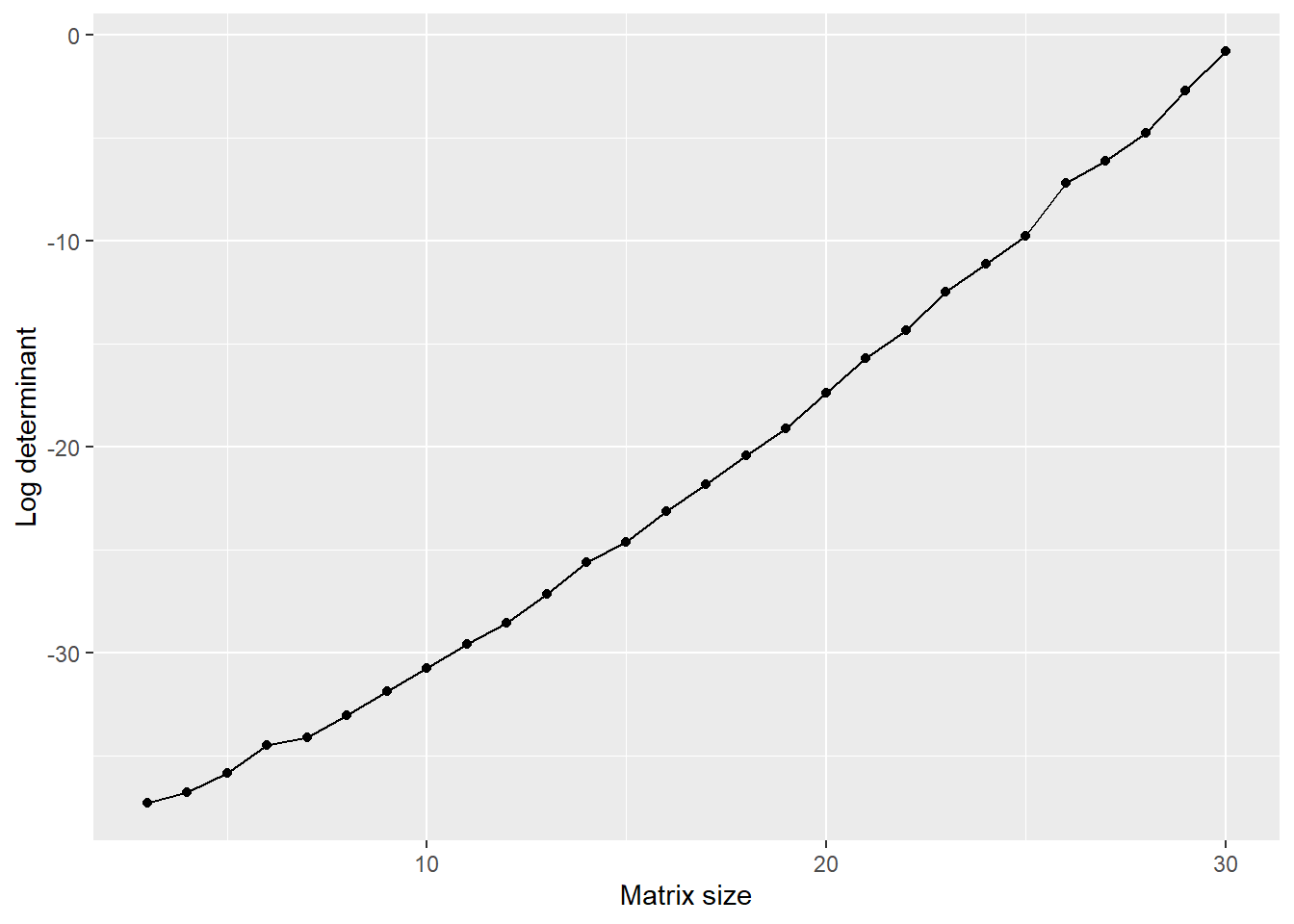

Chapter 12

Exercise 1

# create matrix
m <- 4
A <- matrix(rnorm(m^2), nrow=m, ncol=m)
M <- matrix(0, nrow=m, ncol=m)
G <- matrix(0, nrow=m, ncol=m)

# compute minors matrix
for(i in 1:m){
  for(j in 1:m){
    
    ## select rows and cols
    # implementation matching the original
    rows <- rep(TRUE, m)
    rows[i] <- FALSE
    cols <- rep(TRUE, m)
    cols[j] <- FALSE
    M[i, j] <- det(A[rows, cols])
    
    # a simpler R-version using negative (excluding) indexing
    M[i, j] <- det(A[-i, -j])
    
    # compute G
    G[i, j] <- (-1)^(i + j)
  }
}

# compute C
C <- M * G

# compute A
Ainv <- t(C) / det(A)
AinvI <- solve(A)
round(AinvI - Ainv, 4)

##      [,1] [,2] [,3] [,4]
## [1,]    0    0    0    0
## [2,]    0    0    0    0
## [3,]    0    0    0    0
## [4,]    0    0    0    0

Exercise 2

I renamed T into TM, as T is a logical TRUE in R.

# square matrix
A <- matrix(rnorm(5^2), nrow=5, ncol=5)
Ai <- solve(A)
Api <- pracma::pinv(A)
print(round(Ai - Api))

##      [,1] [,2] [,3] [,4] [,5]
## [1,]    0    0    0    0    0
## [2,]    0    0    0    0    0
## [3,]    0    0    0    0    0
## [4,]    0    0    0    0    0
## [5,]    0    0    0    0    0

# tall matrix
TM <- matrix(rnorm(5*3), nrow=5, ncol=3)
TMl <- solve(t(TM) %*% TM) %*% t(TM)
TMpi <- pracma::pinv(TM)
print(round(TMl - TMpi))

##      [,1] [,2] [,3] [,4] [,5]
## [1,]    0    0    0    0    0
## [2,]    0    0    0    0    0
## [3,]    0    0    0    0    0

Chapter 13

Exercise 2

m <- 4
n <- 4
A <- matrix(rnorm(n=m*n), nrow=m, ncol=n)
Q <- matrix(0, nrow=m, ncol=n)

for(i in 1:n){
  Q[, i] <- A[, i]
  
  # orthogonalize
  a <- A[, i] # convenience
  if (i > 1){
    for(j in 1:(i-1)){
      q <- Q[, j] # convenience
      Q[, i] <- Q[, i] - pracma::dot(a, q) / pracma::dot(q, q) * q 
    }
  }
  
  # normalize
  Q[, i] <- Q[, i] / norm(matrix(Q[, i]), type="F")
}

QR <- qr(A)
Q2 <- qr.Q(QR)

Chapter 14

Exercise 3

# load the data into a table that we convert to a matrix
df <- read.csv("http://sincxpress.com/widget_data.txt", header=FALSE)
data <- as.matrix(df)

# design matrix
X <- cbind(rep(1, nrow(data)), data[, 1:2])
colnames(X) <- c("x1", "x2", "x3")

# outcome variable
y <- data[, 3]

# beta coefficients[]
beta <- lsfit(X, y)$coefficients[1:3]

## Warning in lsfit(X, y): 'X' matrix was collinear

# scaled coefficients (intercept not scaled)
betaScaled <- beta / apply(X, MARGIN=2, FUN=sd)

Exercise 4

library(dplyr)
library(ggplot2)
library(tidyr)

df_long <-
  df %>%
  dplyr::rename("Time of day" = 1, "Age" = 2, "Widgets purchased"=3) %>%
  tidyr::pivot_longer(cols = c("Time of day", "Age"), names_to = "Variable name", values_to = "Variable") %>%
  dplyr::mutate(`Variable name` = factor(`Variable name`, levels=c("Time of day", "Age")))

ggplot(df_long, aes(x = Variable, y=`Widgets purchased`)) + 
  geom_point() + 
  facet_grid(.~`Variable name`, scales="free_x")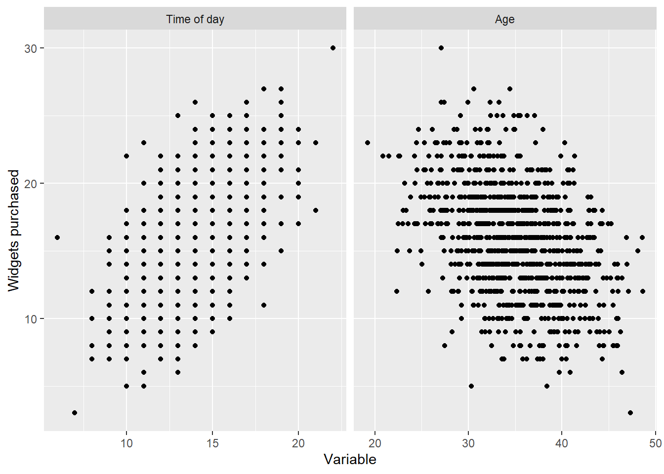

Exercise 5

yHat <- X %*% beta
r2 <- 1 - sum((yHat - y)^2) / sum((y - mean(y))^2)

Chapter 15

Exercise 1

avediffs <- rep(0, times=100)
for(n in 1:100){
  A <- matrix(rnorm(n=n^2), nrow=n, ncol=n)
  B <- matrix(rnorm(n=n^2), nrow=n, ncol=n)
  l1 <- geigen::geigen(A, B, symmetric=FALSE, only.values=TRUE)$values
  l2 <- eigen(solve(B) %*% A)$values
  
  # important to sort eigvals
  l1 <- sort(l1)
  l2 <- sort(l2)
  
  avediffs[n] <- mean(abs(l1-l2))
}

ggplot(data=NULL, aes(x=1:100, y=avediffs)) + 
  geom_point() + 
  xlab("Matrix size") + 
  ylab(expression(paste(Delta, lambda)))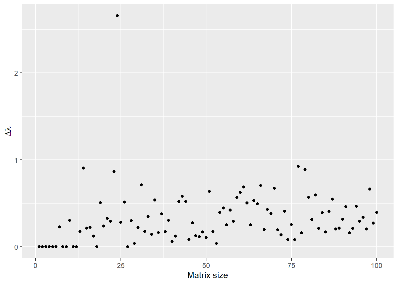

Exercise 2

A <- diag(1:6)
eigenA <- eigen(A)
L <- eigenA$values
V <- eigenA$vectors

Exercise 3

library(dplyr)
library(ggplot2)
library(patchwork)
library(reshape2)

v <- 1:50
lstrow <- c(v[length(v)], v[-length(v)])
H <- pracma::hankel(v, lstrow)
eigH <- eigen(H)
V <- eigH$vectors[, order(eigH$values, decreasing=TRUE)]

# the matrix
plotH <- 
  ggplot(data=reshape2::melt(H), aes(x=1-Var1, y=Var2)) + 
  geom_raster(aes(fill=value), show.legend=FALSE) + 
  labs(title="Hankel matrix") + 
  coord_equal() + xlab("") + ylab("")
  

# eigenvector matrix
plotV <- 
  ggplot(data=reshape2::melt(V), aes(x=Var2, y=Var1)) + 
  geom_raster(aes(fill=value), show.legend=FALSE) + 
  labs(title="Eigenvector matrix") + 
  coord_equal() + xlab("") + ylab("")

# a few eigenvectors
dfV <- 
  data.frame(t(V)) %>%
  dplyr::slice_head(n=4) %>%
  dplyr::mutate(VectorIndex = 1:n()) %>%
  tidyr::pivot_longer(cols = c(X1:X50), names_to="Element", values_to="Value") %>%
  dplyr::group_by(VectorIndex) %>%
  dplyr::mutate(ElementIndex = 1:n()) %>%
  dplyr::select(-Element)

plot4 <- 
  ggplot(data=dfV, aes(x = ElementIndex, y=Value, color=as.factor(VectorIndex))) + 
  geom_line(show.legend=FALSE) + 
  geom_point(show.legend=FALSE) + 
  xlab("Eigenvector element index") + 
  ylab("Eigenvector element value") + 
  labs(title = "First four eigenvectors")

(plotH | plotV) / plot4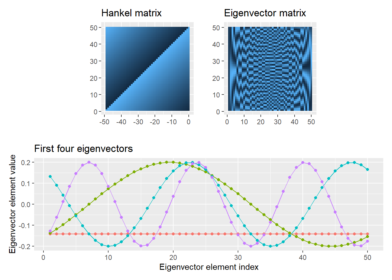

Chapter 16

Exercise 1

In R svd() defaults to “economy” mode. If you want the full matrix, you must specify dimensions for U and V explicitly.

m <- 6
n <- 3
A <- matrix(rnorm(n=m*n), nrow=m, ncol=n)

fullSVD <- svd(A, nu=m, nv=n)
economySVD <- svd(A)

cat(sprintf("Full SVD: (%d, %d), %d, (%d, %d)\n", nrow(fullSVD$u), ncol(fullSVD$u), length(fullSVD$d), nrow(fullSVD$v), ncol(fullSVD$v)))

## Full SVD: (6, 6), 3, (3, 3)

cat(sprintf("Economy : (%d, %d), %d, (%d, %d)\n", nrow(economySVD$u), ncol(economySVD$u), length(economySVD$d), nrow(economySVD$v), ncol(economySVD$v)))

## Economy : (6, 3), 3, (3, 3)

Exercise 2

Note that eigen() sorts eigenvalues and eigenvectors, so sorting is redundant and can be skipped (but I kept it to match the original code).

A <- matrix(rnorm(n=4*5), nrow=4, ncol=5) # matrix
A <- matrix(a, nrow=4, ncol=5, byrow=TRUE)
eigAV <- eigen(t(A) %*% A) 
V <-  eigAV$vectors[, order(eigAV$values, decreasing=TRUE)] # sort descent V
eigAU <- eigen(A %*% t(A)) 
U <-  eigAU$vectors[, order(eigAU$values, decreasing=TRUE)] # sort descent U

# create Sigma
sorted_values <- sort(eigAU$values, decreasing=TRUE)
S <- matrix(0, nrow=nrow(A), ncol=ncol(A))
for(i in 1:length(sorted_values)){
  S[i, i] <- sqrt(sorted_values[i])
}

svdA <- svd(A) # svd

Exercise 3

library(ggplot2)
library(patchwork)
library(RColorBrewer)
library(reshape2)


A <- matrix(rnorm(n=5*3), nrow=5, ncol=3)
svdA <- svd(A)
S <- diag(svdA$d) # need Sigma matrix

fill_palette <- colorRampPalette(rev(brewer.pal(11, "Spectral")))
sc <- scale_colour_gradientn(colours = fill_palette(100), limits=c(min(A), max(A)))


one_layer_plots <- list()
lowrank_plots <- list()
for(i in 1:3) {
  onelayer <- outer(svdA$u[, i], svdA$v[i, ]) * svdA$d[i]
  one_layer_plots[[i]] <- 
    ggplot(data=reshape2::melt(t(onelayer)), aes(x=Var1, y=Var2, fill=value)) + 
    geom_tile(show.legend=FALSE) + theme_void() +
    labs(title=sprintf("Layer %d", i)) +
    coord_equal() + sc
  
  lowrank <- matrix(svdA$u[, 1:i], ncol=i) %*% S[1:i,1:i] %*% t(svdA$v)[1:i,]
  lowrank_plots[[i]] <- 
    ggplot(data=reshape2::melt(t(lowrank)), aes(x=Var1, y=Var2, fill=value)) + 
    geom_tile(show.legend=FALSE) + theme_void() +
    labs(title=sprintf("Layers 1:%d", i)) +
    coord_equal() + sc
}

plotA <- 
  ggplot(data=reshape2::melt(t(A)), aes(x=Var1, y=Var2, fill=value)) + 
  geom_tile(show.legend=FALSE) + theme_void() +
  labs(title="Orig. A") +
  coord_equal() + sc

layout <- "
ABC#
DEFG
"
one_layer_plots[[1]] + one_layer_plots[[2]] + one_layer_plots[[3]] +
  lowrank_plots[[1]] + lowrank_plots[[2]] + lowrank_plots[[3]] + plotA +
  plot_layout(design = layout)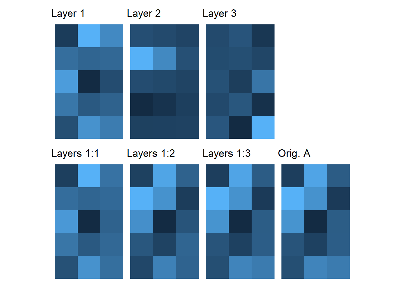

Exercise 4

m <- 6
n <- 16
condnum <- 42

# create U and V from random numbers
U <- qr(matrix(rnorm(m*m), nrow=m, ncol=m))
V <- qr(matrix(rnorm(n*n), nrow=n, ncol=n))

# create singular values vector
s <- seq(condnum, 1, length.out = min(c(m,n)))
S <- diag(s, nrow=m, ncol=n)
# ↓ original code ↓
# S <- matrix(0, nrow=m, ncol=n)
# for(i in 1:min(c(m, n))){
#   S[i, i] <- s[i]
# }

A <- qr.Q(U) %*% S %*% t(qr.Q(V)) # construct matrix
pracma::cond(A)

## [1] 42

Exercise 5

library(imager)

rankN <- 20

picture <- imager::load.image('https://upload.wikimedia.org/wikipedia/en/8/86/Einstein_tongue.jpg')

pic <- as.matrix(picture)
picSVD <- svd(pic, nu=nrow(pic), nv=ncol(pic))
S <- diag(picSVD$d, nrow=nrow(pic), ncol=ncol(pic))

lowrank <- picSVD$u[, 1:rankN] %*% S[1:rankN, 1:rankN] %*% t(picSVD$v)[1:rankN,]

plot(imager::as.cimg(lowrank), axes=FALSE)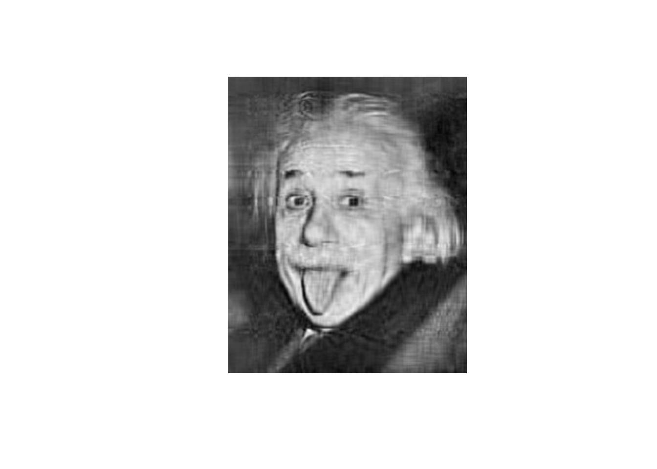

Exercise 6

library(imager)

# convert to percent explained
s <- 100 * picSVD$d / sum(picSVD$d)
ggplot(data=NULL, aes(x=1:100, y=s[1:100])) + 
  geom_line() +
  geom_point() +
  xlab("Component number") +
  ylab("Pct variance explains")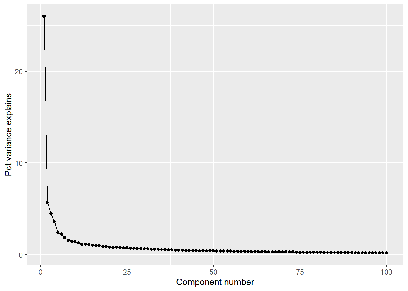

thresh <- 4 # threshold in percent
comps <- s > thresh # comps greater than X%
lowrank <- picSVD$u[, comps] %*% S[comps, comps] %*% t(picSVD$v)[comps,]

layout(t(c(1,2)))
plot(picture, axes=FALSE, main="Original")
plot(as.cimg(lowrank), axes=FALSE, main=sprintf("%s comps with > %g%%", sum(comps), thresh))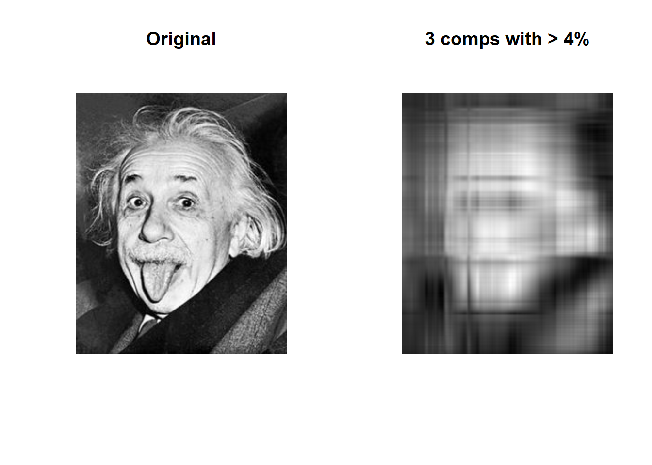

Exercise 7

Note matrix(picSVD$u[, 1:si], ncol=si). Without matrix(, ncol=si), picSVD$u[, 1:si] becomes an atomic vector and matrix multiplication breaks down.

library(ggplot2)

RMS <- rep(0, length(s))
for(si in 1:length(s)){
  lowrank <- matrix(picSVD$u[, 1:si], ncol=si) %*% S[1:si, 1:si] %*% t(picSVD$v)[1:si,]
  diffimg <- lowrank - pic
  RMS[si] <- sqrt(mean(diffimg^2))
}

ggplot(data=NULL, aes(x=1:length(RMS), y=RMS)) + 
  geom_line() + 
  xlab("Rank approximation") + 
  ylab("Error (a.u.)")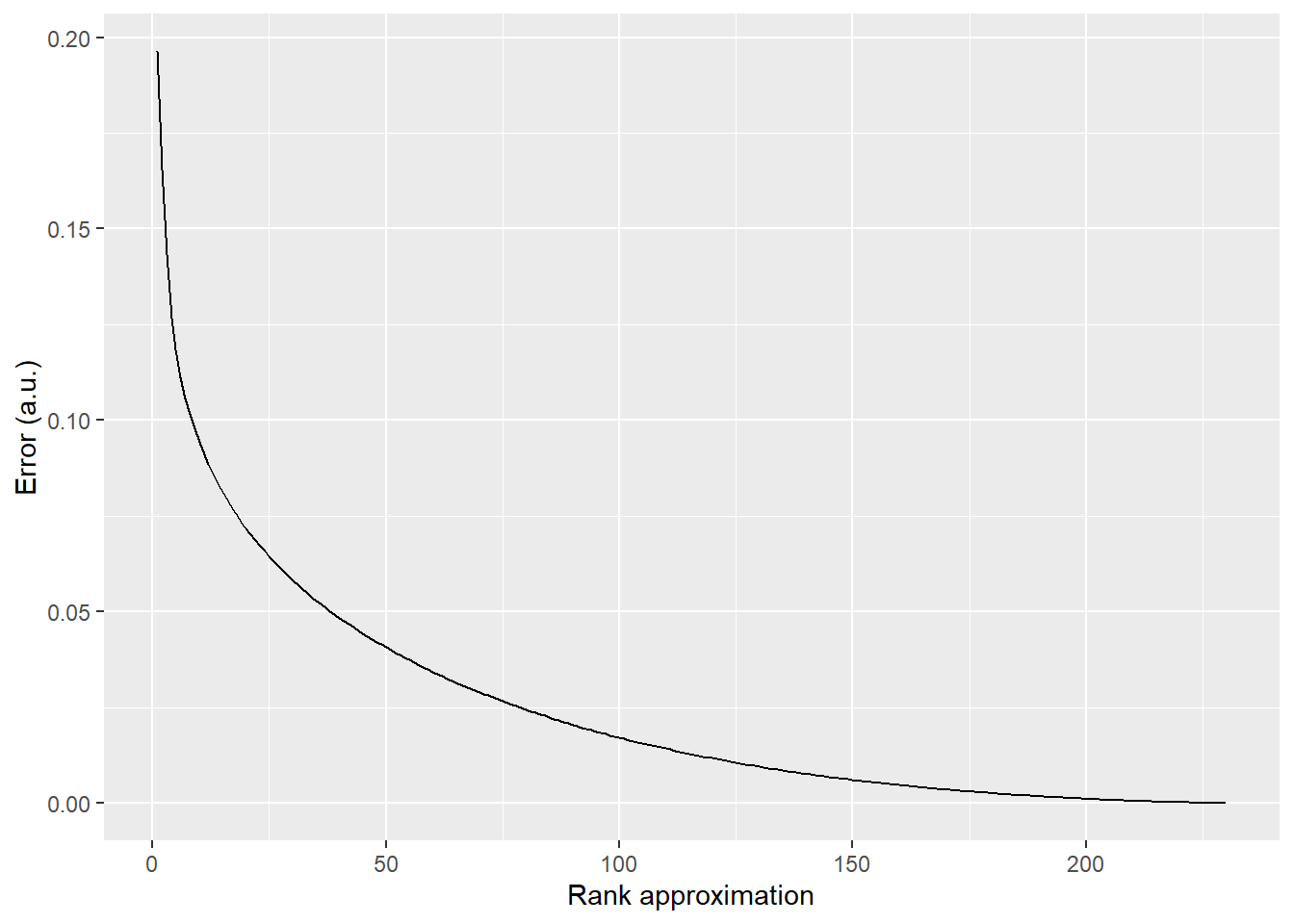

Exercise 8

Reminder, you need to specify nu and nv to ensure full matrices U and V.

library(matrixcalc)

X <- matrix(sample(1:6, size = 4*2, replace = TRUE), nrow=4, ncol=2)
svdX <- svd(X, nu=nrow(X), nv=ncol(X)) # eq. 29
U <- svdX$u
S <- diag(svdX$d, nrow=nrow(X), ncol=ncol(X))
V <- svdX$v

longV1 <- solve(t(U%*%S%*%t(V))%*%U%*%S%*%t(V)) %*% t(U%*%S%*%t(V)) # eq. 30
longV2 <- solve(V%*%t(S)%*%t(U)%*%U%*%S%*%t(V)) %*% t(U%*%S%*%t(V)) # eq. 31
longV3 <- solve(V%*%t(S)%*%S%*%t(V)) %*% t(U%*%S%*%t(V)) # eq. 32
longV4 <- V %*% matrixcalc::matrix.power(t(S) %*% S, -1) %*% t(V)%*%V%*%t(S)%*%t(U) # eq. 33 

MPpinv <- pracma::pinv(X) # eq. 34

Exercise 9

k <- 5
n <- 13
a <- pracma::pinv(matrix(1, nrow=n, ncol=1) * k)
a - 1 / (k * n) # check for zeros

##              [,1]         [,2]         [,3]         [,4]         [,5]
## [1,] 8.673617e-18 6.938894e-18 6.938894e-18 6.938894e-18 6.938894e-18
##              [,6]         [,7]         [,8]         [,9]        [,10]
## [1,] 6.938894e-18 6.938894e-18 6.938894e-18 6.938894e-18 6.938894e-18
##             [,11]        [,12]        [,13]
## [1,] 6.938894e-18 6.938894e-18 6.938894e-18

Exercise 10

M <- 10
cns <- seq(10, 1e10, length.out=30)
avediffs <- rep(0, length(cns))

# loop over condition numbers  
for(condi in 1:length(cns)){
  # create A
  U <- qr.Q(qr(matrix(rnorm(M^2), nrow=M, ncol=M)))
  V <- qr.Q(qr(matrix(rnorm(M^2), nrow=M, ncol=M)))
  S <- diag(cns[condi], nrow=M, ncol=M)
  A <- U %*% S %*% t(V) # construct matrix 

  # create B
  U <- qr.Q(qr(matrix(rnorm(M^2), nrow=M, ncol=M)))
  V <- qr.Q(qr(matrix(rnorm(M^2), nrow=M, ncol=M)))
  S <- diag(cns[condi], nrow=M, ncol=M)
  B <- U %*% S %*% t(V) # construct matrix 
  
  # GEDs and sort
  l1 <- sort(eigen(A)$values)
  l2 <- sort(eigen(B)$values)
  
  avediffs[condi] <- mean(abs(l1-l2))
}

ggplot(data=NULL, aes(x=cns, y=avediffs)) + 
  geom_line() + 
  xlab("Cond. number") + 
  ylab(expression(paste(Delta, lamda)))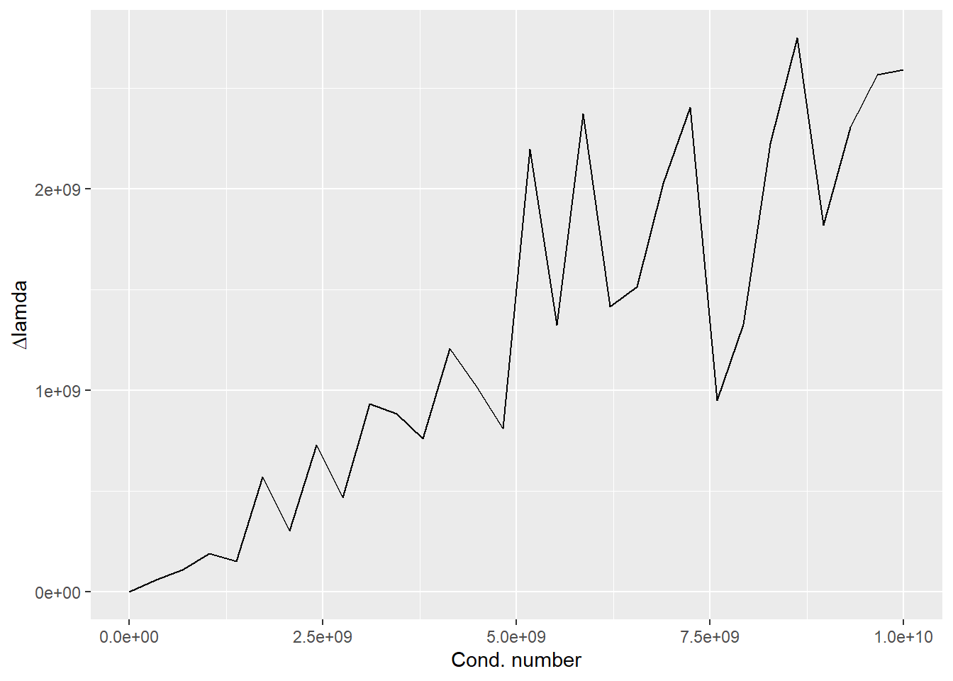

## Chapter 17 ### Exercise 1 {-}

library(plotly)

A <- matrix(c(-2, 3, 2, 8), nrow=2, ncol=2, byrow=TRUE)
vi <- seq(-2, 2, step=0.1)
quadform <- matrix(0, nrow=length(vi), ncol=length(vi))

for(i in 1:length(vi)){
  for(j in 1:length(vi)){
    v <- matrix(c(vi[i], vi[j]), ncol=1)
    quadform[i, j] <- t(v) %*% A %*% v / (t(v) %*% v)
  }
}
  
plot_ly(z = quadform, type = "surface")

Exercise 2

n <- 4
nIterations <- 500
defcat <- rep(0, nIterations)

for(iteri in 1:nIterations){
  # create matrix
  A <- matrix(sample(-10:10, size=n^2, replace=TRUE), nrow=n, ncol=n)
  e <- eigen(A)$values
  while (is.complex(e)){
    A <- matrix(sample(-10:10, size=n^2, replace=TRUE), nrow=n, ncol=n)
    e <- eigen(A)$values
  }
  
  # "zero" threshold (from rank)
  t <- n * pracma::eps(max(svd(A)$d))
  
  # test definiteness
  if (all(sign(e) == 1)) {
    defcat[iteri] <- 1 # pos. def
  }
  else if (all(sign(e)>-1 & (sum(abs(e)<t)>0))){
    defcat[iteri] <- 2 # pos. semidef
  }
  else if (all(sign(e)<1 & (sum(abs(e)<t)>0))){
    defcat[iteri] <- 4 # neg. semidef
  }
  else if (all(sign(e) == -1)) {
    defcat[iteri] <- 5 # neg. def
  }
  else {
    defcat[iteri] <- 3 # indefinite
  }
}

# print out summary
for(i in 1:5)
{
  print(sprintf("cat %d: %d", i, sum(defcat == i)))
}

## [1] "cat 1: 1"
## [1] "cat 2: 0"
## [1] "cat 3: 498"
## [1] "cat 4: 0"
## [1] "cat 5: 1"

Chapter 18

Exercise 1

n <- 200
X <- matrix(rnorm(n*4), nrow=n, ncol=4) # data
X <- apply(X, MARGIN=2, FUN=scale, scale=FALSE) # mean-center
covM <- t(X) %*% X / (n-1) # covariance
stdM <- solve(diag(apply(X, MARGIN=2, FUN=sd))) # stdevs
corM <- stdM %*% t(X) %*% X %*% stdM / (n - 1) # R

# compare ours against R's
print(round(covM - cov(X), 3))

##      [,1] [,2] [,3] [,4]
## [1,]    0    0    0    0
## [2,]    0    0    0    0
## [3,]    0    0    0    0
## [4,]    0    0    0    0

print(round(corM - cor(X), 3))

##      [,1] [,2] [,3] [,4]
## [1,]    0    0    0    0
## [2,]    0    0    0    0
## [3,]    0    0    0    0
## [4,]    0    0    0    0

Chapter 19

Exercise 1

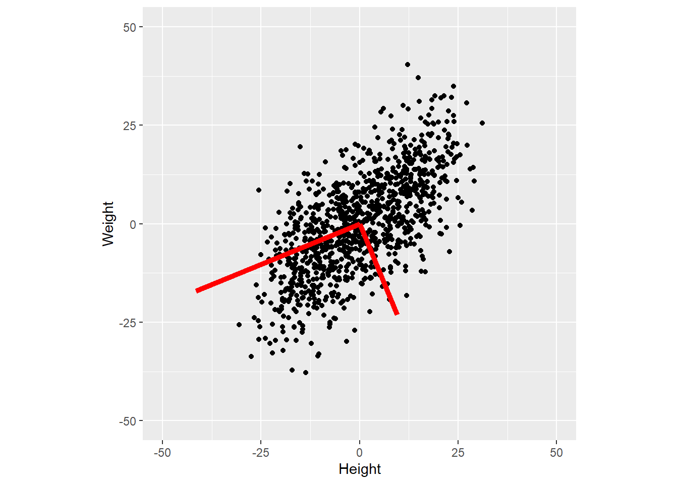
library(ggplot2)

# create data
N <- 1000
h <- rnorm(n=N, mean = seq(150, 190, length.out = N), sd=5)
w <- h * .7 - 50 + rnorm(N, mean=0, sd=10)

# covariance
X <- cbind(h, w)
X <- apply(X, MARGIN=2, scale, scale=FALSE)
C <- t(X) %*% X / (length(h) - 1)

# PCA
eigC <- eigen(C)

# sorting below is redundant in R, as values and vectors are presorted
i <- order(eigC$values, decreasing=TRUE) 
V <- eigC$vectors[, i]
eigvals <- eigC$values[i]
eigvals <- 100 * eigvals / sum(eigvals)
scores <- X %*% V # not used, but useful code

# plot data with PCs
ggplot(data=NULL, aes(x = X[, 1], y = X[, 2])) + 
  geom_point() + 
  geom_segment(aes(x=0, y=0, xend=V[1, 1] * 45, yend=V[2, 1] * 45), color="red", size=2) +
  geom_segment(aes(x=0, y=0, xend=V[1, 2] * 25, yend=V[2, 2] * 25), color="red", size=2) +
  scale_x_continuous(name="Height", limits=c(-50, 50)) + 
  scale_y_continuous(name="Weight", limits=c(-50, 50)) + 
  coord_equal()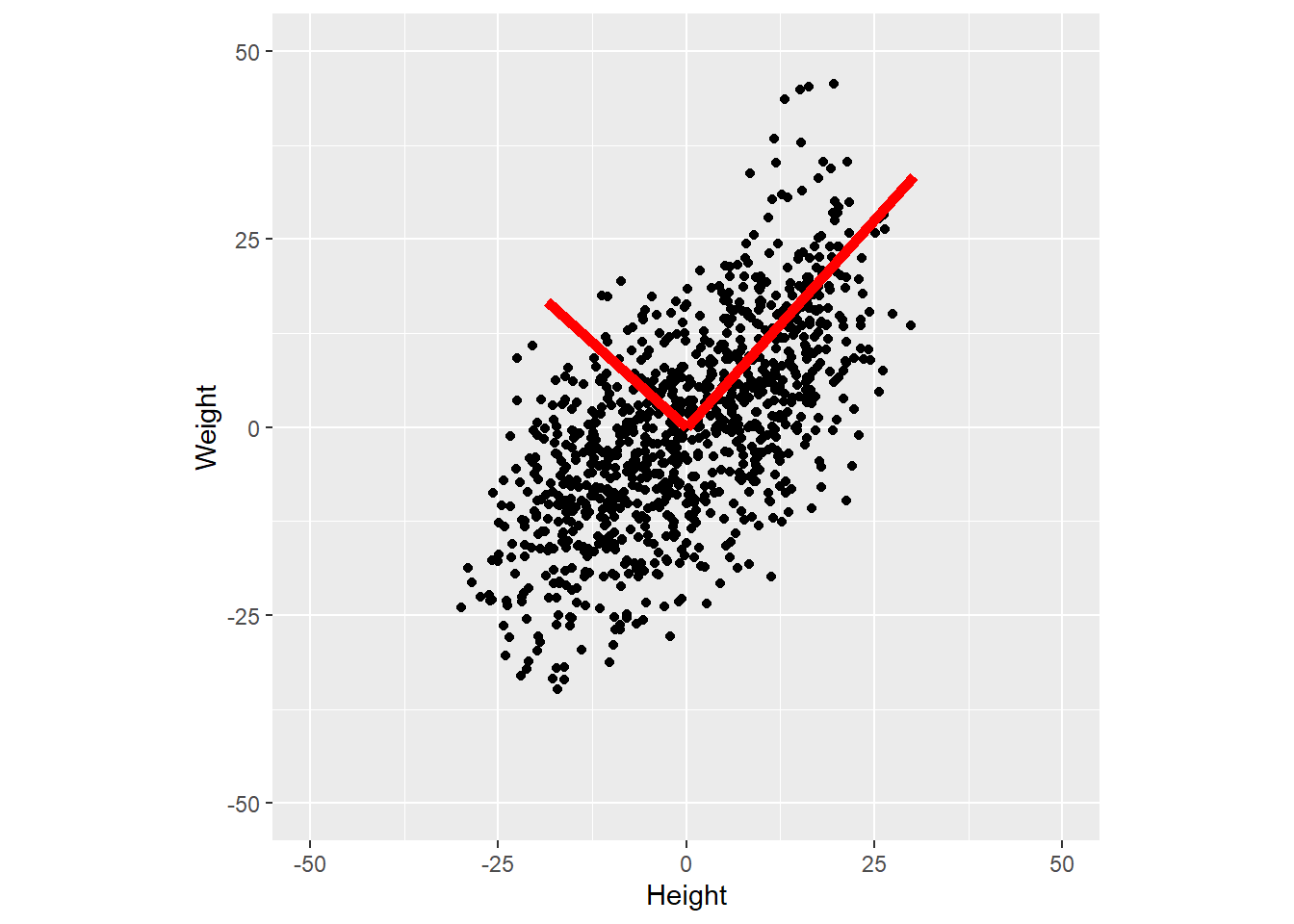

Exercise 2

X <- apply(X, MARGIN=2, scale, scale=FALSE)
svdX <- svd(X, nu=nrow(X), nv=ncol(X))
scores <- X %*% svdX$v
s <- diag(svdX$d)^2 / (nrow(X) - 1)
s <- 100 * s / sum(s) # s == eigvals

Exercise 3

library(ggplot2)

# create data
N <- 1000
h <- rnorm(n=N, mean = seq(150, 190, length.out = N), sd=5)
w <- h * .7 - 50 + rnorm(N, mean=0, sd=10)

# covariance
X <- cbind(h, w)
C <- t(X) %*% X / (length(h) - 1)

# PCA
eigC <- eigen(C)

# sorting below is redundant in R, as values and vectors are presorted
i <- order(eigC$values, decreasing=TRUE) 
V <- eigC$vectors[, i]
eigvals <- eigC$values[i]
eigvals <- 100 * eigvals / sum(eigvals)
scores <- X %*% V # not used, but useful code

# now we center the data
X <- apply(X, MARGIN=2, scale, scale=FALSE)

# plot data with PCs
ggplot(data=NULL, aes(x = X[, 1], y = X[, 2])) + 
  geom_point() + 
  geom_segment(aes(x=0, y=0, xend=V[1, 1] * 45, yend=V[2, 1] * 45), color="red", size=2) +
  geom_segment(aes(x=0, y=0, xend=V[1, 2] * 25, yend=V[2, 2] * 25), color="red", size=2) +
  scale_x_continuous(name="Height", limits=c(-50, 50)) + 
  scale_y_continuous(name="Weight", limits=c(-50, 50)) + 
  coord_equal()