13 (Generalized) Linear regression and Resampling
As I have warned you at the very beginning, this seminar will not teach you statistics. The latter is a big topic in itself and, in my experience, if you know statistics and you know which specific tool you need, figuring out how to use it in R is fairly trivial (just find a package that implements the analysis and read the docs). Conversely, if your knowledge of statistics is approximate, knowing how to call functions will do you little good. The catch about statistical models is that they are very easy to run (even if you implement them by hand from scratch) but they are easy to misuse and very hard to interpret77.
To make things worse, computers and algorithms do not care. In absolute majority of cases, statistical models will happily accept any input you provide, even if it is completely unsuitable, and spit out numbers. Unfortunately, it is on you, not on the computer, to know what you are doing and whether results even make sense. The only solution to this problem: do not spare any effort to learn statistics. Having a solid understanding of a basic regression analysis will help you in figuring out which statistical tools are applicable and, even more importantly, which will definitely misguide you. This is why I will give an general overview with some examples simulations but I will not explain here when and why you should use a particular tool or how to interpret the outputs. Want to know more? Attend my Bayesian Statistics seminar or read an excellent Statistical Rethinking by Richard McElreath that the seminar is based on.
Grab exercise notebook before reading on.
13.1 Linear regression: simulating data
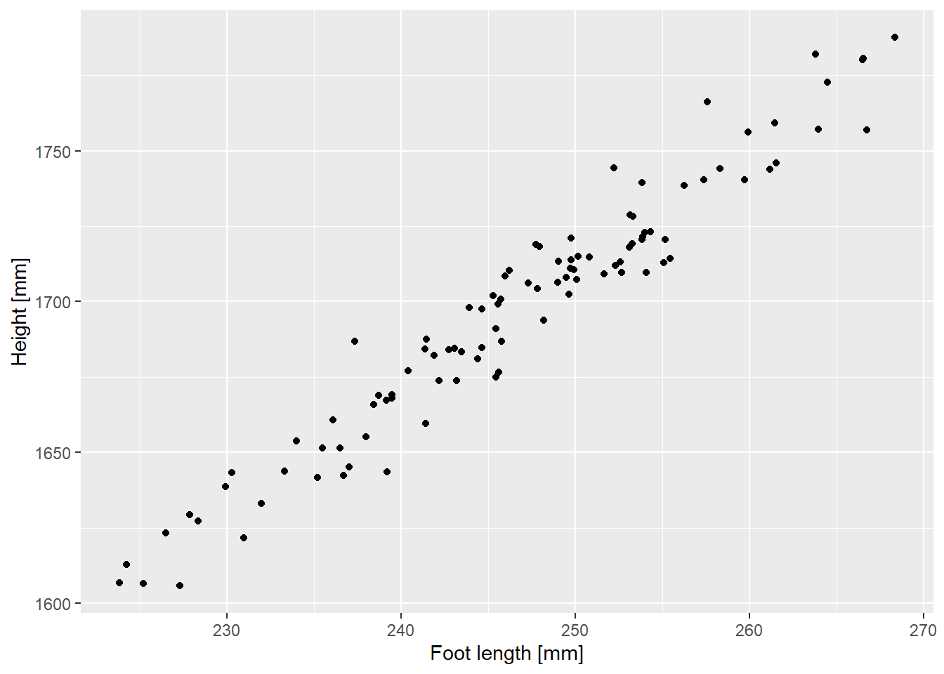
Our first statistical model will be linear regression. When you experiment with analysis, it is easier to notice if something goes wrong if you already know the answer. Which is why let us simulate the data with a linear relationship in it: overall height versus foot length. A conference paper I have found online suggests that foot length distribution is 246.726±10.3434 mm (mean and standard deviation, assume normal distribution) and the formula for estimate height is \(Height = 710 + 4 \cdot Foot + \epsilon\)78 where \(\epsilon\) (residual error) is normally distributed around the zero with a standard deviation of 10. Generate the data (I used 100 points) putting it into a table with two columns (I called them FootLength and Height) and plot them to match the figure below. You can set seed to 826 to replicate me exactly.
Do exercise 1.
13.2 Linear regression: statistical model
Let us use a linear regression model to fit the data and see how accurately we can estimate both intercept and slope terms. R has a built-in function for linear regression model — lm() — that uses a common formula design to specify relationship. This formula approach is widely used in R due to its power and simplicity. The syntax for a full factorial linear model with two predictors is y ~ x1 + x2 + x1:x2 where individual effects are added via + and : mean “interaction” between the variables. There are many additional bells and whistles, such as specifying both main effects and an interaction of the variables via asterisk (same formula can be compressed to y ~ x1 * x2) or removing an intercept term (setting it explicitly to zero” y ~ 0 + x1 * x2). You can see more detail in the online documentation but statistical packages frequently expand it to accommodate additional features such as random effects. However, pay extra attention to the new syntax as different packages may use different symbols to encode a certain feature or, vice versa, use the same symbol for different features. E.g., | typically means a random effect but I was once mightily confused by a package that used it to denote variance term instead.
Read the documentation for lm() and summary() functions. Fit the model and print out the full summary for it. Your output should look like this
##
## Call:
## lm(formula = Height ~ FootLength, data = height_df)
##
## Residuals:
##      Min       1Q   Median       3Q      Max
## -24.0149  -7.0855   0.7067   6.0991  26.6808
##
## Coefficients:
##              Estimate Std. Error t value Pr(>|t|)
## (Intercept) 721.26822   24.12584   29.90   <2e-16 ***
## FootLength    3.95535    0.09776   40.46   <2e-16 ***
## ---
## Signif. codes:  0 '***' 0.001 '**' 0.01 '*' 0.05 '.' 0.1 ' ' 1
##
## Residual standard error: 10.13 on 98 degrees of freedom
## Multiple R-squared:  0.9435, Adjusted R-squared:  0.9429
## F-statistic:  1637 on 1 and 98 DF,  p-value: < 2.2e-16
As you can see, our estimate for the intercept term is fairly close 725±24 mm versus 710 mm we used in the formula. Same goes for the foot length slope: 3.95±0.1 versus 4.
Do exercise 2.
I think it is nice to present information about the model fit alongside the plot, so let us prepare summary about both intercept and slope terms in a format estimate [lower-97%-CI-limit..upper-97%-CI-limit]. You can extract estimates themselves via coef() function and and their confidence intervals via confint(). In both cases, names of the terms are specified either as names of the vector or rownames of matrix. Think how would you handle this. My approach is to convert matrix with confidence intervals to a data frame (converting directly to tibble removes row names that we need later), turn row names into a column via rownames_to_column(), convert to a tibble so I can rename ugly converted column names, add estimates as a new column to the table, and relocate columns for a consistent look. Then, I can combine them into a new variable via string formatting (I prefer glue). You need one(!) pipeline for this. My summary table looks like this
| Term | Estimate | LowerCI | UpperCI | Summary |
|---|---|---|---|---|
| (Intercept) | 721.268216 | 668.139580 | 774.396852 | (Intercept): 721.27 [668.14..774.4] |
| FootLength | 3.955354 | 3.740062 | 4.170646 | FootLength: 3.96 [3.74..4.17] |
Do exercise 3.
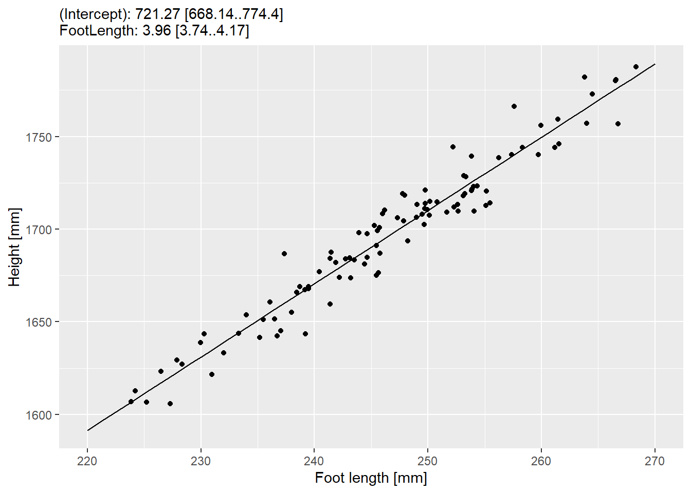
Statistical model is only as good as its predictions, so whenever you fit a statistical model to the data, you should compare its predictions to the data visually. ggplot2 provides an easy solution to this via geom_smooth() that you have met earlier. For didactic purposes, let us use a slightly longer way of generating predictions ourselves and plotting them alongside the data. R provides a simple interface to generating prediction for a fitted model via predict() function: you pass a fitted model to it and it will generate prediction for every original data point. However, you can also generate data for data points not present in the data (so-called “counterfactuals”) by passing a table to newdata parameter. We will use the latter option. Generate a new table with a single column FootLength (or, however you called it in the original data) with a sequence of number going from the lowest to the highest range of our values (from about 220 to 270 in my case) in some regular steps (I picked a step of 1 but think of whether choosing a different one would make a difference). Pass this new data as newdata to predict, store predictions in the Height column (now the structure of your table with predictions matches that with real data) and use it with geom_line(). Here’s how my plot looks like.
Do exercise 4.
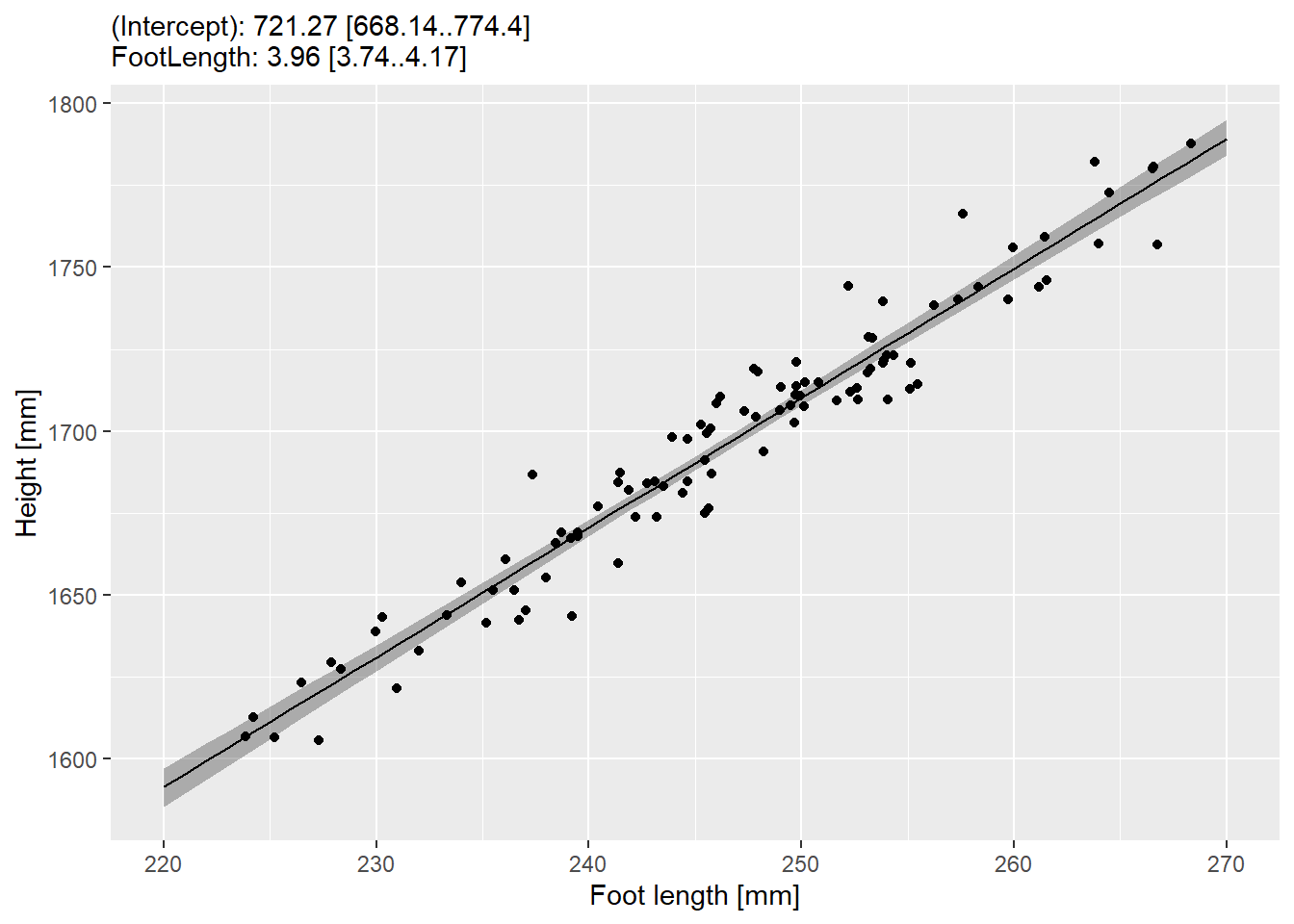
We can see the trend, but when working with statistical models, it is important to understand uncertainty of its predictions. For this, we need to plot not just the prediction for each foot length but also the confidence interval for the prediction. First, we will do it an easy way as predict() function has options for that as well via its interval parameter (we want "confidence"). Use it to generate 97% confidence interval for each foot length you generated and plot it as a geom_ribbon().

Do exercise 5.
13.3 Linear regression: bootstrapping predictions
Let us replicate these results but use bootstrap approach, which will work even when you don’t have a convenience function. One iteration consists of:
- Randomly sample original data table with replacement.
- Fit a linear model to that data.
- Generate predictions for the interval, the same way we did above, so that you end up with a table of
FootLength(going from 220 to 270) and (predicted)Height.
Write the code and put it into a function (think about which parameters it would need). Test it by running it the function a few times. Values for which column should stay the same or change?
Do exercise 6.
Once you have this function, things are easy. All you need is to follow the same algorithm as for computing and visualizing confidence intervals for the Likert scale:
- Call function multiple times recording the predictions (think map() and list_rbind())
- Compute 97% confidence interval for each foot length via quantiles
- Plot them as geom_ribbon() as before.
Do exercise 7.
13.4 Logistic regression: simulating data
Let us practice more but this time we will using binomial data. Let us assume that we measure success in playing video games for people drank tea versus coffee (I have no idea if there is any effect at all, you can use liquids of your liking for this example). Let us assume that we have measure thirty participants in each group and average probability of success was 0.4 for tea and 0.7 for coffee79 groups. You very much know the drill by now, so use rbinom() (you want twenty 0/1 values, so figure out which size and which n you need) to generate data for each condition, put it into a single table with 60 rows (bind_rows() might be useful) and two columns (Condition and Success). Your table should look similar to this (my seed is 12987)
| Condition | Success |
|---|---|
| Tea | 0 |
| Tea | 1 |
| Tea | 1 |
| Tea | 0 |
| Tea | 1 |
Do exercise 8.
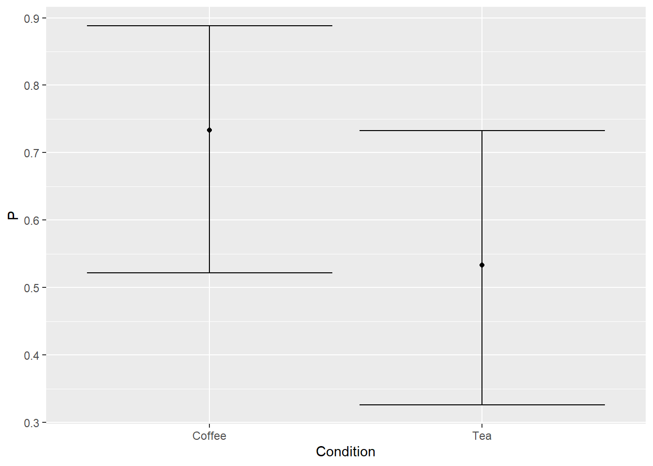
Now, let us visualize data. You need to compute average and 97% confidence interval for each condition. The average is easy (divide total number of successes for condition by total number of participants) but confidence interval is trickier. Luckily for us, package binom has us covered. It implements multiple methods for computing it. I used binom.exact() (use ?binom.exact in the console to read the manual, once you loaded the library). You plot should look like this (or similar, if you did not set seed). Note that our mean probability for Tea condition is higher than we designed it (sampling variation!) and confidence intervals are asymmetric. The latter is easier to see for the coffee condition (redo it with probability of success 0.9 to make it more apparent) and is common for data on limited interval.
Do exercise 9.
13.5 Logistic regression: fitting data
Let us fit the data using generalized linear models — glm — with "binomial" family. That latter bit and the name of the function are the only new bits, as formula works the same way as in lm(). Print out the summary and it should look like this.
##
## Call:
## glm(formula = Success ~ Condition, family = "binomial", data = game_df)
##
## Coefficients:
##              Estimate Std. Error z value Pr(>|z|)
## (Intercept)    1.0116     0.4129   2.450   0.0143 *
## ConditionTea  -0.8781     0.5517  -1.592   0.1115
## ---
## Signif. codes:  0 '***' 0.001 '**' 0.01 '*' 0.05 '.' 0.1 ' ' 1
##
## (Dispersion parameter for binomial family taken to be 1)
##
##     Null deviance: 78.859  on 59  degrees of freedom
## Residual deviance: 76.250  on 58  degrees of freedom
## AIC: 80.25
##
## Number of Fisher Scoring iterations: 4
Do exercise 10.
Note that this is logistic regression, so the estimates need are harder to interpret. Slope term for condition Tea is in the units of log-odds and we see that it is negative, meaning that model predict fewer successes in tea than in coffee group. Intercept is trickier as you need inverted logit function (for example, implemented as inv.logit() in boot package) to convert it to probabilities. Here, 0 corresponds to probability of 0.5, so 1 is somewhere above that. Personally, I find these units very confusing, so to make sense of it we need to use estimates (coef() functio will work here as well) to compute scores for each condition and then tranlate them to probabilities via inv.logit(). Coffee is our “baseline” group (simple alphabetically), so \(logit(Coffee) = Intercept\) and \(logit(Tea) = Intercept + ConditionTea\). In statistics, link function is applied to the left side, but we apply its inverse to the right side. I just wanted to show you this notation, so you would recognize it the next time you see it.
Your code should generate a table with two columns (Condition and P for Probability). It should look like this
| Condition | P |
|---|---|
| Coffee | 0.7333333 |
| Tea | 0.5333333 |
Do exercise 11.
13.6 Logistic regression: bootstrapping uncertainty
Let us bootstrap predicted probability of success following the template we used already twice but with a slight twist. Write a function (first write the inside code, make sure it works, then turn it into a function) that samples our data, fits the model, generates and returns model with prediction. The only twist is that we will sample each condition separately. sample_frac() but you will need to group data by condition before that. Also, pass iteration index (the one you are purrring over) as a parameter to the function and store in a separate column Iteration. This will allows us to identify individual samples, making it easier to compute the difference between the conditions later on.
Repeat this computation 1000 times and you will end up with a table with two columns (Condition and P) and 2000 rows (1000 per condition). Instead of computing aggregate information, visualize distributions using geom_violin(). Here’s how the plot should look like.
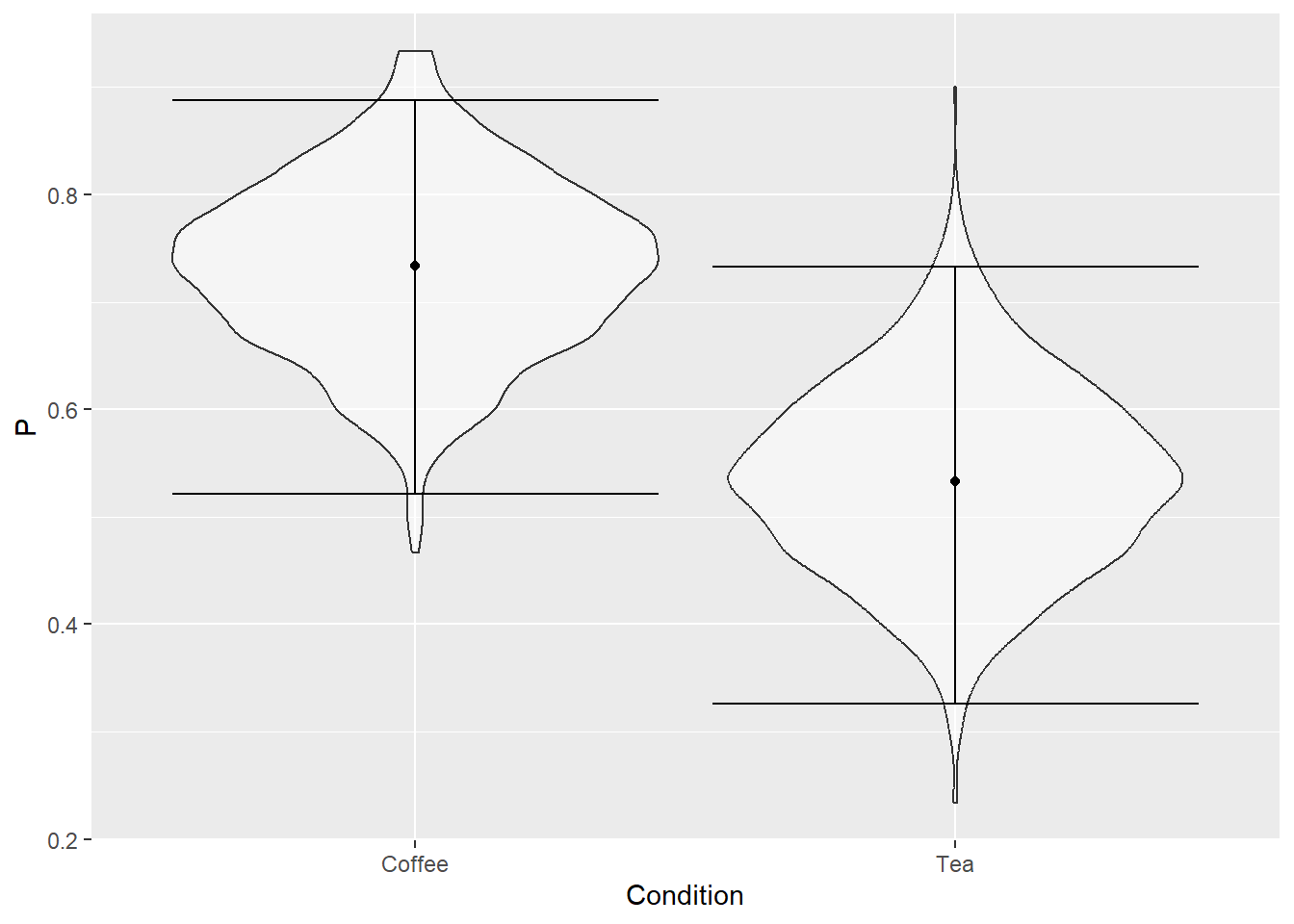
Do exercise 12.
As a final step, let us compute average and 97% confidence interval for the difference between the conditions. You have the samples but in a long format, so you need to make table wide, so you will end up with three columns: Iteration, Coffee, andTea`. Compute a new column with difference between tea and coffee, compute and nicely format the statistics putting into the figure caption. Hint: you can pull the difference column out of the table to make things easier.
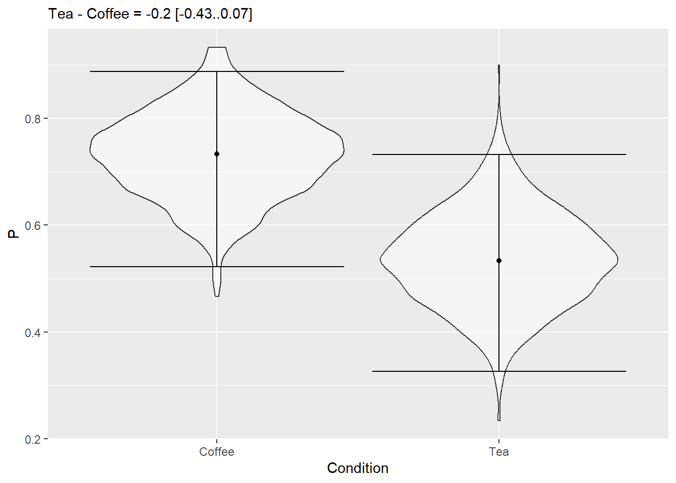
Do exercise 13.