Because the gaze samples tend to be noisy, different methods use various approaches for computing velocity from noisy samples. Methods by Engbert and Kliegl (2003) and Otero-Millan et al. (2014) used the same approach based on averaging over multiple samples to compute velocity, whereas Nyström and Holmqvist (2010) compute a simple derivative and then filter it. By default, package uses the former approach (velocity_function = diff_ek) but you can also use the latter (velocity_function = diff_nh) or implement a custom method (see below). Acceleration is computed the same way but from velocity samples.
Differentiation following Engbert and Kliegl (2003)
This method computes velocity over a predefined time window controlled via ek_velocity_time_window that defaults to 20 ms. The width of the window is converted to samples based on the sampling_rate parameter and is ensured to be an odd number equal to or larger than 3. I.e., for a window that is three samples long, the velocity is computed based on one sample before and one sample after the current, for a five-samples window - two samples before and after, etc. The code always starts with the requested window size but all iteratively reduces it by two samples to accommodate for trial limits and missing values. An NA velocity is returned only if even the smallest window (three samples wide) cannot be used.
In general, horizontal and vertical velocity components are computed as \[v_x[i] = \frac{\sum_{j=1}^{(N-1)/2}x[i+j] - x[i-j]}{\sum_{j=1}^{(N-1)/2}2j\cdot\Delta t}\] where \(i\) is the index of a sample, \(\Delta t = \frac{1}{sample~rate}\) is a duration of a single sampling frame, and \(N\) is an odd integer width of the moving average used to compute the velocity. In Engbert and Kliegl (2003), \(N=5\) and \(\Delta t = 4\) (250 Hz sampling rate) translate into a 20 ms moving average window (default value used in the method implementation). Below is a derivation that shows the equivalence of the formula above to formula 1 in Engbert and Kliegl (2003). For \(N=5\): \[\frac{\sum_{j=1}^{(5-1)/2}x[i+j] - x[i-j]}{\sum_{j=1}^{(5-1)/2}2j\cdot\Delta t}=\] \[\frac{\sum_{j=1}^{2}x[i+j] - x[i-j]}{\sum_{j=1}^{2}2j\cdot\Delta t}=\]
\[\frac{x[i+1] - x[i-1]+x[i+2] - x[i-2]}{2\Delta t + 4\Delta t}=\] \[\frac{x[i+2] + x[i+1] - x[i-1] - x[i-2]}{6\Delta t}\]
Differentiation following Nyström and Holmqvist (2010)
Horizontal and vertical components of velocity are computed from adjacent samples, the amplitude is computed from the components and then is filtered using the Savitzky-Golay filter. Filter order is controlled via nh_sg_filter_order option and defaults to 2.
Comparing two methods
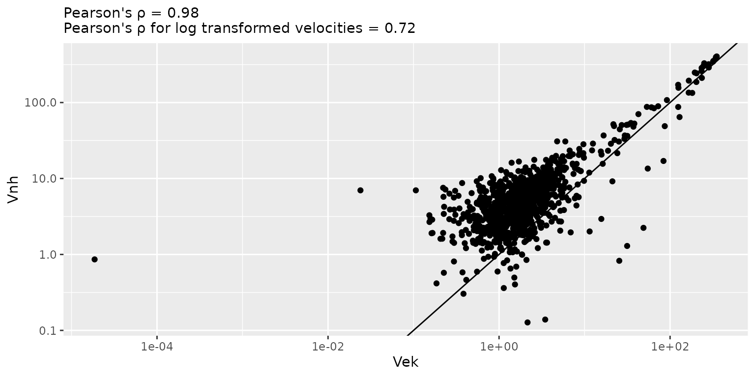
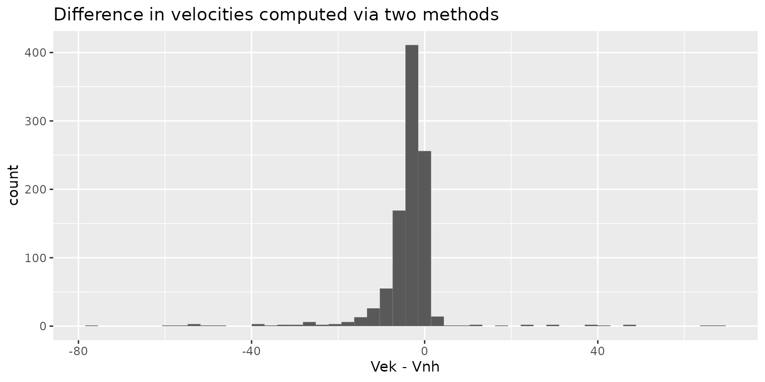
The two methods produce comparable but different velocity values. However, this has only a minor effect on saccade detection, see a vignette on Using sample votes.
# computing velocity using two methods
vel_ek <- saccadr::diff_ek(x = single_trial$x,
                           y = single_trial$y,
                           trial = rep(1, nrow(single_trial)),
                           sample_rate = 500)
vel_nh <- saccadr::diff_nh(x = single_trial$x,
                           y = single_trial$y,
                           trial = rep(1, nrow(single_trial)),
                           sample_rate = 500)
vel_comparison <- na.omit(data.frame(EK = vel_ek[['amp']], NH = vel_nh[['amp']])) %>%
  dplyr::filter(NH > 0) %>% # values can be negative due to filtering
  dplyr::mutate(logEK = log(EK), logNH = log(NH))

# plotting amplitude comparison
pearson_rho <- cor(vel_comparison[['EK']], vel_comparison[['NH']])

ggplot(data = vel_comparison, aes(x = EK, y = NH)) +
  geom_abline() +
  geom_point() +
  scale_x_log10() +
  scale_y_log10() +
  labs(subtitle = sprintf("Pearson's ρ = %.2f\nPearson's ρ for log transformed velocities = %.2f", pearson_rho, cor(vel_comparison[['logEK']], vel_comparison[['logNH']])),
       x = "Vek",
       y = "Vnh")
# plotting
ggplot(data = NULL, aes(x = vel_comparison[['EK']] - vel_comparison[['NH']])) +
  geom_histogram(bins = 50) +
  xlab("Vek - Vnh") +
  labs(title = "Difference in velocities computed via two methods")
Implementing and using a custom differentiation function
A custom function should be as a follows
diff_custom <- function(x, y,  trial, sample_rate, options=NULL) {
  # compute vertical and horizontal components
  df <- data.frame(x = ..., # differentiate values of x
                   y = ...) # differentiate values of y

  # compute amplitude
  df[['amp']] = sqrt(df[['x']]^2 + df[['y']]^2))

  # return a data.frame with columns x, y, and amp
  return(df)
}
Arguments that are passed to the function (all vectors have the same length):
-
x,yvectors with values, either x and y gaze coordinates or velocity components (for acceleration). -
sample_ratescalar value in Hz. -
trialvector with trial index per sample. -
optionsa named list with method-specific options. See the example below for how to use them. See alsooption_or_default()function.
The function must return a data.frame with three columns: x (horizontal component), y (vertical component), and amp (amplitude).
Here is an example of a simple velocity function that respects trial borders
library(dplyr)

diff_custom <- function(x, y,  trial, sample_rate, options=NULL) {
  # computing frame time step
  delta_t_s <- 1 / sample_rate

  # --- differentiate (compute velocity or acceleration) and filter
  data.frame(trial = trial,
             x = x,
             y = y) %>%

    # compute velocity and acceleration for each trial
    group_by(trial) %>%
    mutate(x = (x - lag(x)) / delta_t_s,
           y = (y - lag(y)) / delta_t_s,
           amp = sqrt(x^2 + y^2))
}
And here is a similar function but that uses an optional custom_velocity_lag parameter so that it can be different from 1
diff_lag_n <- function(x, y,  trial, sample_rate, options=NULL) {
  # obtain lag or use default
  lag_n <- saccadr::option_or_default(options, "custom_velocity_lag", 1)

  # computing frame time step
  delta_t_s <- 1 / sample_rate

  # --- differentiate (compute velocity or acceleration) and filter
  data.frame(trial = trial,
             x = x,
             y = y) %>%

    # compute velocity and acceleration for each trial
    group_by(trial) %>%
    mutate(x = (x - lag(x, lag_n)) / delta_t_s,
           y = (y - lag(y, lag_n)) / delta_t_s,
           amp = sqrt(x^2 + y^2))
}
References
Engbert, Ralf, and Reinhold Kliegl. 2003. “Microsaccades uncover the orientation of covert attention.” Vision Research 43 (9): 1035–45. https://doi.org/10.1016/S0042-6989(03)00084-1.
Nyström, Marcus, and Kenneth Holmqvist. 2010. “An adaptive algorithm for fixation, saccade, and glissade detection in eyetracking data.” Behavior Research Methods 42 (1): 188–204. https://doi.org/10.3758/BRM.42.1.188.
Otero-Millan, J., Jose L Alba Castro, Stephen L Macknik, and S. Martinez-Conde. 2014. “Unsupervised clustering method to detect microsaccades.” Journal of Vision 14 (2): 18–18. https://doi.org/10.1167/14.2.18.