9 Instrumental Variables
Disclaimer
My understanding is that instrumental variables are unicorns. They are immensely powerful and can magically turn an observational study into, effectively, a randomize experiment enabling you to infer causality. But they are rare, perhaps, even rarer than unicorns themselves, which is why most example you find are based on the same (or very similar) data.They are also often described as a source of “natural randomization”, yet, the best examples I have found (effect of military experience on career/wages, effect of studying in a charter school on math skills) involved deliberate randomization in a form of lottery that you can conveniently use.
Can we estimate an effect of military experience on wages
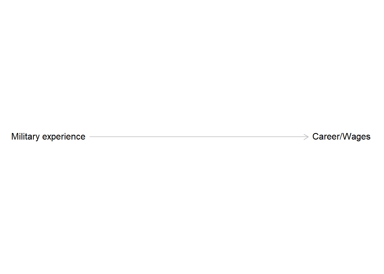
One of the examples, which you can find online, is an effect of military experience on wages. Conceptually, everything is simple, you just want to know a direct effect of military experience on wages.
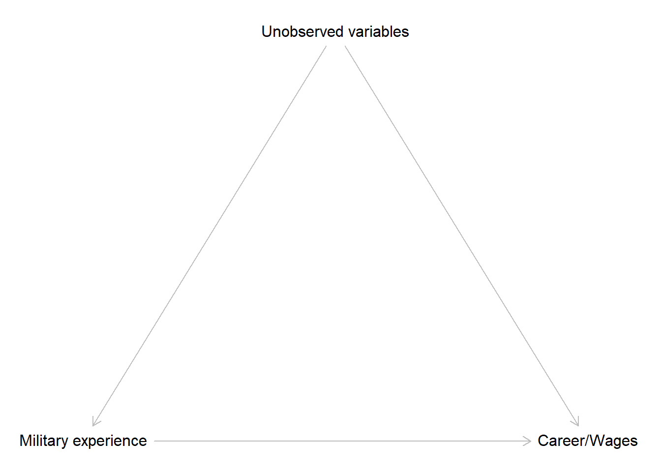
However, in practice both a decision to join military and choices of career can be cause by the same set of unobserved factors. If you come from a family with military background, this will affect both your decision join military and the kind of career you want to pursue. If you are patriotic and want to serve the country, you might opt for both military and lower-earning career in public sector. Conversely, if you are interested in becoming a successful lawyer, going into military might be more of a hindrance than of help. In short, we have a backdoor path through unobserved variables and we have no easy way to close it.
Draft as an instrumental variable
If we would be able to perform a randomized experiment, things would be easy: Take similar people and randomly send / not send them to military, observe the effect of this on their career and wages. Now, we cannot do it but, perhaps, we can find a situation it was actually done and use it for our advantage. This makes the whole situation a sort of a hybrid: we observe an outcome of randomization that someone else did for their own purposes
In this case, during the Vietnam war people were drafted based on their assigned draft numbers. The latter were determined by your date of birth but the relationship between the birth day within a year and the draft number was randomized through the lottery. In addition, the order within a day was randomized through lottery of initials. The purpose was to create a perfect randomization where any background (apart from you being male and being eligible for military service) had no effect on whether or not your were drafted. And, although the lottery was created to address inequalities, it created an almost perfect randomized experiment for us to use. Almost, because some people with early numbers avoided being drafted through various means, whereas some people with later draft numbers volunteered and were enlisted.
The DAG it creates is the following
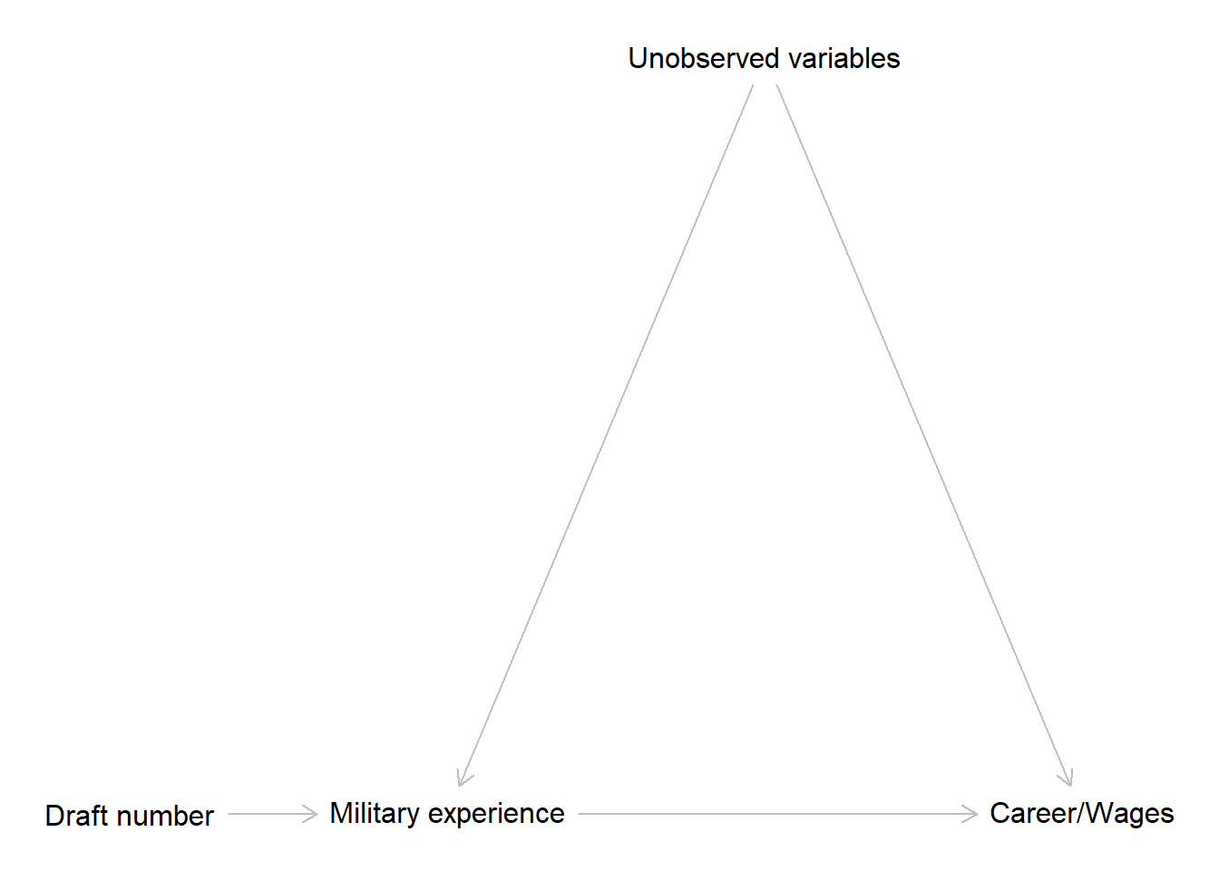
As you can see, we are still not able to close the backdoor path between military experience and wages because the randomization is not perfect. You will see how we can still overcome this problem using two-stage least squares (the default approach you find almost everywhere, referred to as “two-stage worst squares” by McElreath) and using covariance of residuals (as in the book).
Two-stage least squares
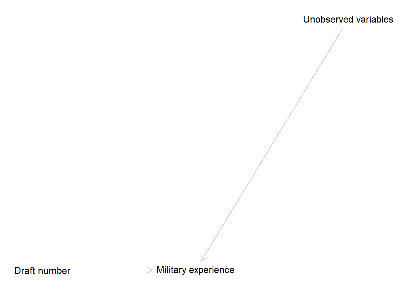
The main idea is two split our DAG into two halves and estimated the effects one by one, hence, “two-stage”. First, use draft number to predict the military experience.
The linear model is \[ME \sim Normal(\widehat{ME}, \sigma_{ME})\\ \widehat{ME} = \alpha_{ME} + \beta_{DN} \cdot DN\]
where \(\alpha_M\) is an arbitrary intercept term, \(\beta_{DN}\) encode the main effect of draft number, and \(\sigma\) is the standard deviation of residuals. You can also write the same model in a different format, which you are likely to encounter in other tutorials and lectures: \[\widehat{ME} = \alpha_{ME} + \beta_{DN} \cdot DN + \epsilon_{ME}\] Here, the difference between the predicted military experience (note the hat above \(\widehat{ME}\)) and the actual one is described by \(\epsilon_{ME}\): residuals that come from a normal distribution that is centered at 0 with standard deviation of \(sigma_{ME}\), which is implicit in this format. Note that both versions express same variables and encode the same dependence but differ in whether the residuals (\(epsilon\)) or the standard deviation of the distribution they come from (\(sigma\)) are implicit or explicit.
As draft number is independent from unobserved variables due to the lottery, the predicted military experience is also independent from them. All the dependence gets transferred to the residuals instead, because residuals are variance that our signal cannot explain (that point will become important later on).
Now, for the second stage, we use predicted military experience, as it is independent of the unobserved variables and, therefore, we do not need to close the backdoor path!
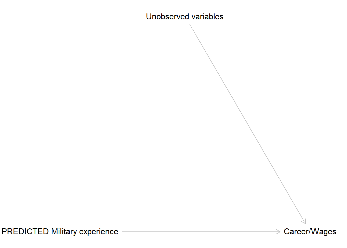
The model is, again, simple but do note that in two-stage least squares we are using predicted military experience \(\widehat{ME}\)! \[CW \sim Normal(\widehat{CW}, \sigma_{CW})\\ \widehat{CW} = \alpha_{CW} + \beta_{ME} \cdot \widehat{CW}\\ or\\ \widehat{CW} = \alpha_{CW} + \beta_{ME} \cdot \widehat{ME} + \epsilon_{CW} \]
Again, all the dependence between unobserved variables and career/wages gets offloaded into the residuals \(\epsilon_{CW}\) and you get you nice and clean direct effect of predicted military experience. Importantly, for you interpretation you equate the effect of the predicted military experience with an effect of an actual one. This is, of course, one big elephant in the room because you need to be certain that \(\widehat{ME}\) is indeed accurate. Unfortunately, if it is not, your inferences are incorrect and you are back to square one.
Covarying residuals
This is the approach presented in the book that allows you to use actual military experience as a predictor and still solve the problem of the backdoor path. The initial idea is the same: Let us use our instrumental variable to compute a “pure” military experience, uncontaminated by unobserved variables.
\[\widehat{ME} = \alpha_{ME} + \beta_{DN} \cdot DN + \epsilon_{ME}\]
Again, all the variance due to unobserved variables is accumulated by residuals (\(\epsilon_{ME}\)), which are correlated with them. The latter part is trivially true because residuals are always correlated with “noise”, precisely because we defined it as influence of unobserved variables we did not measure and, therefore, cannot explicitly account for. If we could measure and include them, we would observe same correlation explicitly. Alas, we did not measure them and, therefore, in our typical model the fact that residuals are correlated with unobserved variables is of no immediate practical value (beyond checking for their exchangeability).
Now, imagine that we could compute not just a prediction from our first stage but a pure randomized military experience that is not correlated with unobserved variables. Obviously, we cannot, otherwise we would not worry about the backdoor path, but what do we know about a linear model that includes that magic pure randomized military experience as a predictor? That its true direct effect on career/wages will be independent from unobserved variables and, therefore, all their influence will be offloaded into residuals (\(\epsilon_{\widehat{CW}}\), note the hat that differentiates them the residuals that you get if you use observed military experience), which will be correlated with those unobserved variables. Just like the residuals of our first stage model (\(\epsilon_{ME}\))! But if both sets of residuals are correlated with unobserved variables (\(\epsilon_{ME} \propto UV\) and \(\epsilon_{\widehat{CW}} \propto UV\)), the two sets of residuals are also correlated: \(\epsilon_{ME} \propto \epsilon_{\widehat{CW}}\).
These correlated residuals sound wonderfully entertaining but why should we care about them given that \(\epsilon_{\widehat{CW}}\) are hypothetical residuals given the hypothetical randomized military experience that we do not have access to? Because we can make them real by using their covariance with \(\epsilon_{ME}\) that we can compute! Here is the idea: let us use two simple linear models to predict military experience from draft number and career/wages from actual military experience but allow the residuals of two models to be correlated. Again, given that \(\epsilon_{ME} \propto UV\), if we make \(\epsilon_{ME} \propto \epsilon_{CW}\), therefore, \(\epsilon_{CW} \propto UV\). In other words, \(\epsilon_{CW} \approx \epsilon_{\widehat{CW}}\). But this means that since \(\epsilon_{CW}\) accounts for the variance due to unobserved variables, it must not be accounted for by other terms of the linear model and our effect of military experience (\(\beta^{true}_{ME}\)) expresses just the direct path: \[\widehat{CW} = \alpha_{CW} + \beta^{true}_{ME} \cdot ME + \epsilon_{\widehat{CW}}\]
This is a very elegant trick: We do not know what the correlation between residuals and unobserved variables is but we do know that it must be the same (very similar) and we account for it by enforcing the correlation between the residuals that we deduced must exist. On the one hand, there is an obvious elephant in the room in that the whole thing works well only if the assumption that residuals are correlated is true. On the other hand, because we are fitting the covariance matrix as part of the model, we can check whether our assumption about that correlation was supported by data. If it was not, our instrumental variable was probably not as good as hoped for.