8 Mixtures

8.1 Beta Binomial

Beta binomial is defined as a product of binomial and beta distributions. \[BetaBinomial(k|N, p, \theta) = Binomial(k|N,p) \cdot Beta(p|\beta_1, \beta_2),\] where \(k\) is number of successes (e.g., “heads” in a coin toss), \(N\) is total number of trials/draws, and \(p\) is the probability of success), and \(\beta_1\) and \(\beta_2\) determine the shape of the beta distribution. The book uses reparametrized version of the beta distribution, sometimes called beta proportion: \[BetaBinomial(k|N, p, \theta) = Binomial(k|N,p) \cdot Beta(p|p, \theta),\] where \(\theta\) is precision parameter. \(p\) and \(\theta\) can be computed from \(\beta_1\) and \(\beta_2\) as \[ p = \frac{\beta_1}{\beta_1 + \beta_2}\\ \theta = \beta_1 + \beta_2 \] The latter form makes it more intuitive but if you look at the code of dbetabinom(), you will see that you can use shape1 and shape2 parameters instead of probe and theta.

Recall the (unnormalized) Bayes rule (\(p\) is probability, \(y\) is an outcome, \(...\) parameters of the prior distribution): \[ Pr(p | y) = Pr(y | p) \cdot Pr(p | ...) \] Examine the formula again and you can see that you can think about beta binomial as a posterior distribution for a binomial likelihood with the beta distribution as prior for parameter \(p'\) of the binomial distribution:

\[BetaBinomial(N, p, \theta | k) = Binomial(k|N,p) \cdot Beta(p| p_{mode}, \theta)\]

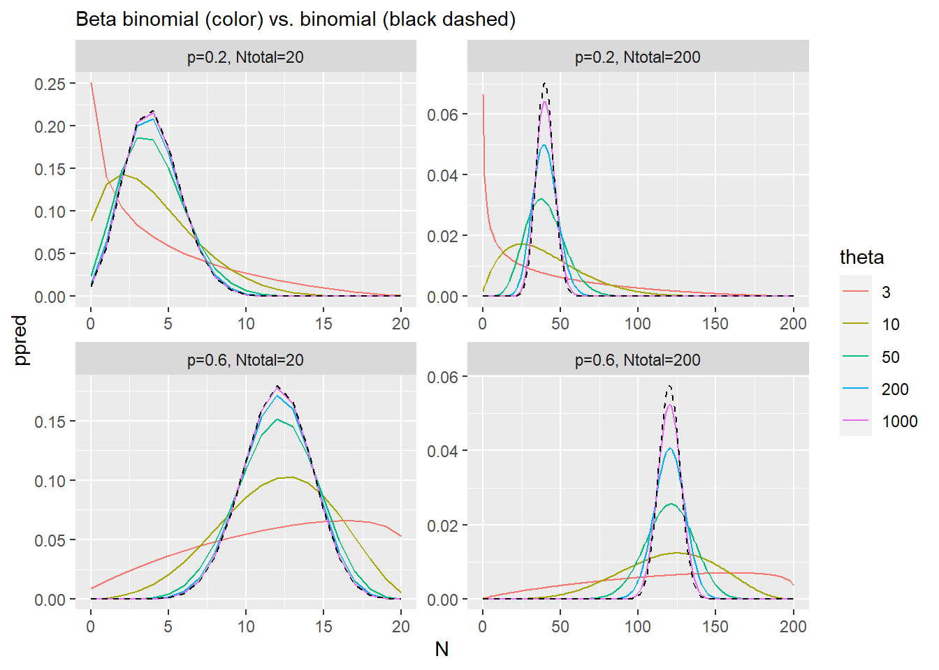
Thus, beta binomial is a combination of all binomial distributions weighted by a beta distribution that has its mode at \(p_{mode}\) and its width is determined by \(\theta\). In other words, when we use binomial distribution alone, we state that we can compute the probability directly as \(p = \text{some linear model}\). Here, we state that our knowledge is incomplete and, at best, we can predict mode of the beta distribution from which this probability comes from and we let data determine variance/precision (\(\theta\)) of that distribution. Thus, our posterior will reflect two uncertainties based on two loss functions: one about the number of observed events (many counts are compatible with a given \(p\) but with different probabilities), as for the binomial, plus another one about \(p\) itself (many values of \(p\) are compatible with given \(p_{mode}\) and \(\theta\)). This allows model to compute a trade-off by considering values of \(p\) that are less likely from prior point of view (they are away from \(p_{mode}\)) but that result in higher probability of \(k\) given that chosen \(p\). We will see the same trick again later in the book, when we will use it to incorporate uncertainty about measured value (i.e., at best, we can say that the actual observed value comes from a distribution with that mean and standard deviation).

In practical terms, this means that parameter \(\theta\) controls the width of the distribution (see plots below). As \(\theta\) approaches positive infinity, our prior uncertainty about \(p\) is reduced to zero, which means that we now consider only one binomial distribution, where \(p' = p\), which is equivalent to the simple binomial distribution. Thus, beta binomial at most is as narrow as the binomial distribution.

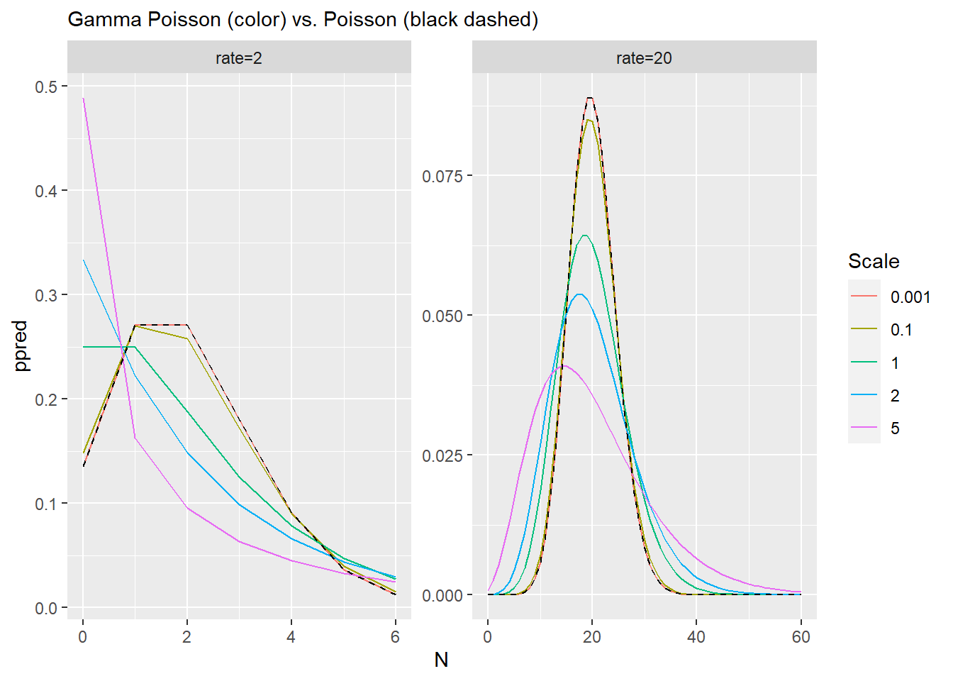
8.2 Negative binomial, a.k.a. Gamma Poisson

The idea is the same: We do not have enough information to compute the rate of events, so instead, we compute the mean of the Gamma distribution rates come from and let data determine its variance (scale). Again, in practical terms this means that for the smallest scale our uncertainty about the rate is minimal and distribution matches the Poisson processes with a fixed rate. Any increase in uncertainty (larger values for scale parameter), mean broader distribution that is capable to account for more extreme values.

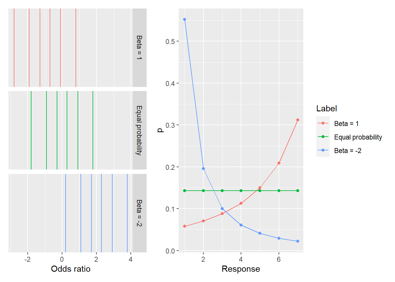
8.3 Ordered categorical

From log odds to logit link. \[ log(\frac{Pr(y_i \leq k)}{1 - Pr(y_i \leq k)}) = \alpha_k \\ \frac{Pr(y_i \leq k)}{1 - Pr(y_i \leq k)} = e^{\alpha_k} \\ Pr(y_i \leq k) = e^{\alpha_k} \cdot ( 1 - Pr(y_i \leq k)) \\ Pr(y_i \leq k) \cdot ( 1 + e^{\alpha_k}) = e^{\alpha_k} \\ Pr(y_i \leq k) = \frac{e^{\alpha_k}}{1 + e^{\alpha_k}} \]

df_p <-
  tibble(alpha = seq(-10, 10, length.out=100)) %>%
  mutate(p = exp(alpha) / (1 + exp(alpha)))

ggplot(df_p, aes(x=alpha, y=p)) + 
  geom_line()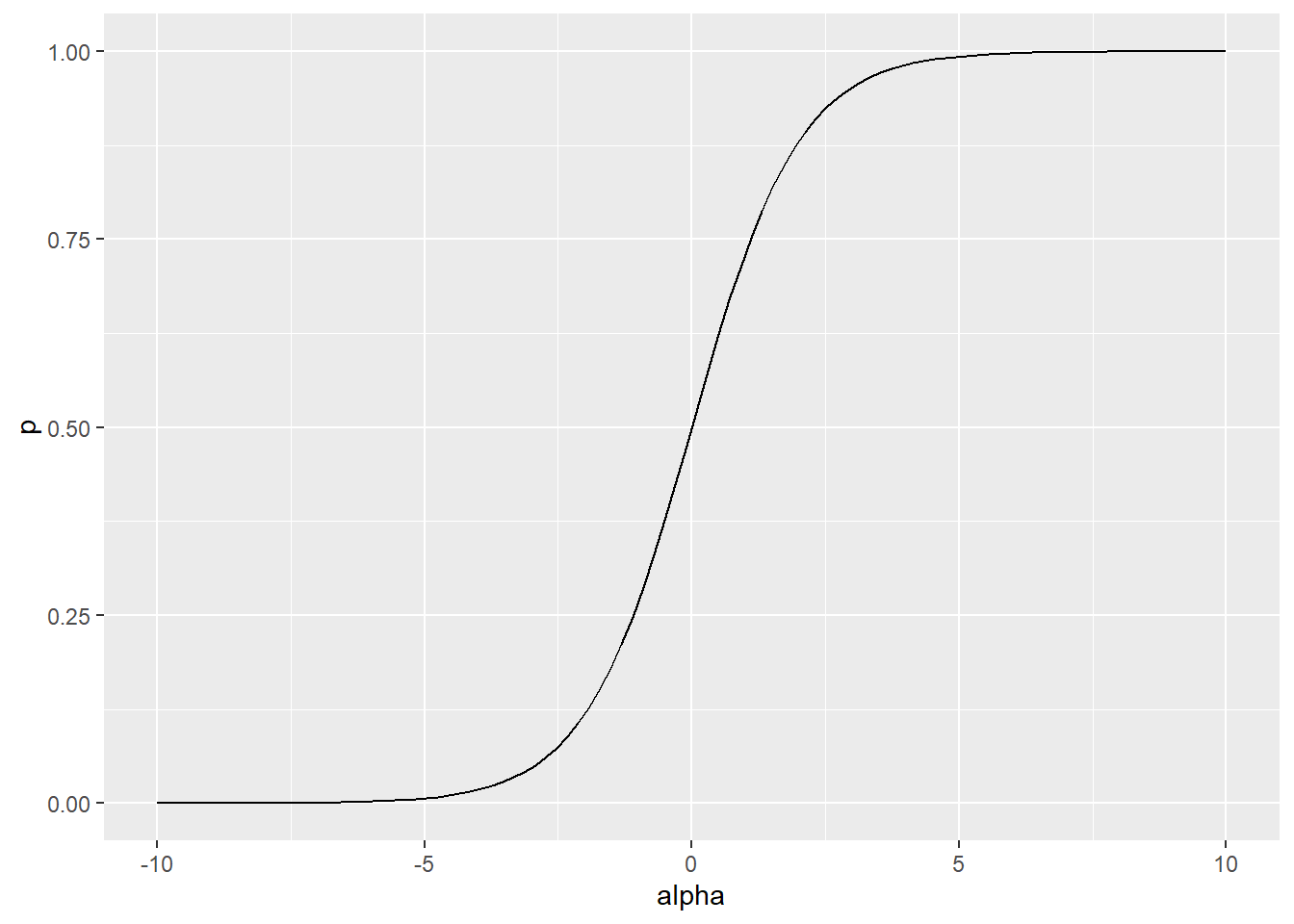

equal_probability <- log(((1:6) / 7) /  (1 - (1:6) / 7))
  
df_ord_cat <- 
  tibble(Response = 1:7, 
         p = rethinking::dordlogit(1:7, 0, equal_probability),
         Label = "Equal probability") %>%
  bind_rows(tibble(Response = 1:7, 
         p = rethinking::dordlogit(1:7, 0, equal_probability - 1),
         Label = "Beta = 1")) %>%
  bind_rows(tibble(Response = 1:7, 
         p = rethinking::dordlogit(1:7, 0, equal_probability + 2),
         Label = "Beta = -2")) %>%
  mutate(Label = factor(Label, levels = c("Beta = 1", "Equal probability", "Beta = -2")))

df_cuts <-
  tibble(Response = 1:6, 
         K = equal_probability,
         Label = "Equal probability") %>%
  bind_rows(tibble(Response = 1:6, 
         K = equal_probability - 1,
         Label = "Beta = 1")) %>%
  bind_rows(tibble(Response = 1:6, 
         K = equal_probability + 2,
         Label = "Beta = -2")) %>%
  mutate(Label = factor(Label, levels = c("Beta = 1", "Equal probability", "Beta = -2")))
  

cuts_plot <-
  ggplot(data=df_cuts,) + 
  geom_vline(aes(xintercept = K, color=Label), show.legend = FALSE) +
  facet_grid(Label~.) +
  scale_x_continuous("Odds ratio")

prob_plot <- 
  ggplot(data=df_ord_cat, aes(x=Response, y=p, color=Label)) + 
  geom_point() + 
  geom_line()

cuts_plot + prob_plot